Add Timeseries

Before we can forecast the operational income of the coffee shop, we need to account for another detail in our case study. Remember:

John and Jack believe they’ll need 10 weeks to set-up their new shop in the leased property.

In other words, it will take 10 weeks before they may sell their first coffee and start satisfying the demand that we calculated in the previous section using the Distribution node. For that reason, we are going to add in a Timeseries node that models the months in operation (for more information on Timeseries nodes click here).

1. From the Palette, click and drag a Timeseries node onto the design surface.
2. Rename the node Fraction of Month Operating.
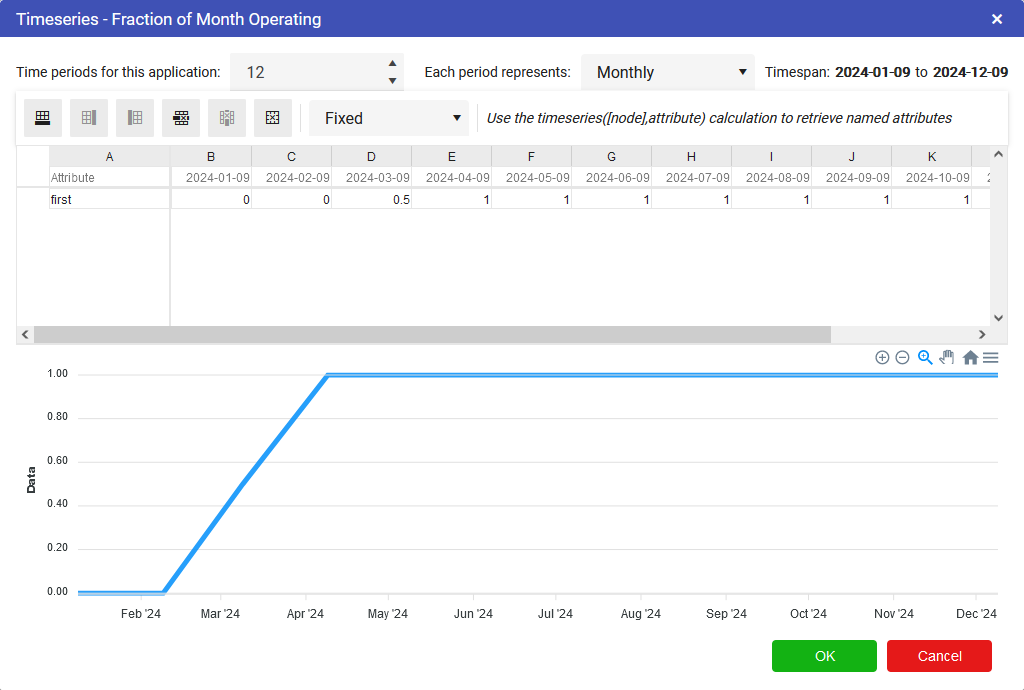
3. Click on the Timeseries value (currently 0.00) to open the timeseries editor.
4. At the top of the Timeseries editor, set the number of periods to 12 and set the periods to represent monthly.
5. Enter 0.5 into the Timeseries excel cell D2 and 1 into the cells E2 through to M2, then press OK.
   Info

   The editor supports excel-like dragging of values across cell. Select the little blue circle of the cell marker for this purpose.

   

We now have our Timeseries node now, so we can now work out the monthly income while the Coffee Shop is in Operation.

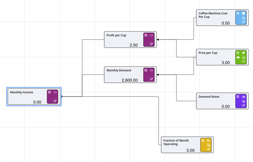
1. Add a new Calculation node to the left of your previous calculations and rename it to Monthly Income.

   Info

   You can use the mouse to click and drag to pan around the driver model, or the scroll wheel of your mouse to zoom in and out if you start to run out of space on this page.

2. Connect the timeseries and the other two calculations (Profit per Cup and Monthly Demand) to the new Calculation node.

3. Set the expression for the new calculation to: [Fraction of Month Operating] * [Monthly Demand] * [Profit per Cup].

4. Confirm the driver model looks like.

We now have a forecast of the operational income for John’s coffee shop. Now that we have this we can go and model the fixed overhead costs.