Akumen Basics
Learning the Ropes
This chapter will guide you through the basics of the Akumen layout.
This chapter will guide you through the basics of the Akumen layout.
The Akumen main page consists of three sections:
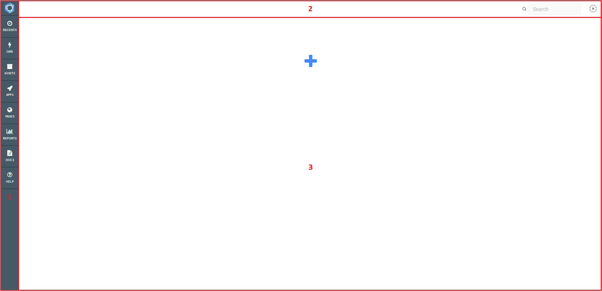

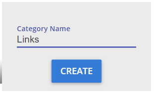
Click the plus icon
 Type in your category name and click “CREATE”
When hovering over a category, there are 4 icons that appear in the top right corner
 These icons are:
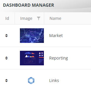
To change the order that categories appear on the dashboard:
The sidebar contains nine links:

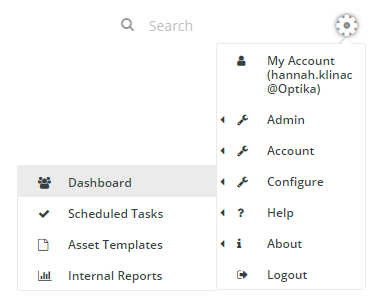
Settings are located under the cog icon at the top-right corner of the screen.
This provides you with a number of administration functions. These functions are for advanced users.
Depending on your permission level, you will be able to see and access different administrative areas within the settings menu.
Under Help, you can Raise a Ticket. Raising a support ticket will generate an email to support@idoba.com, which you can also email directly, about any issue or query you may have.
Selecting Logout from this menu will close your Akumen session.
To the left of the settings cog is the search box.
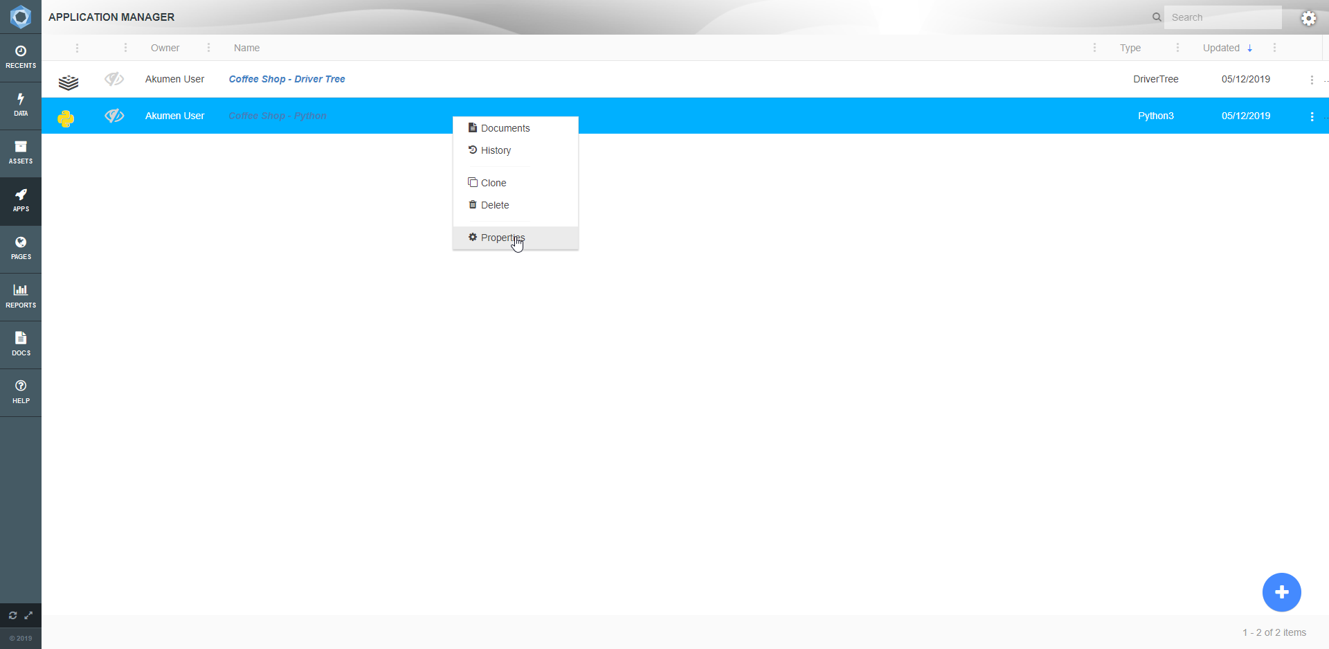
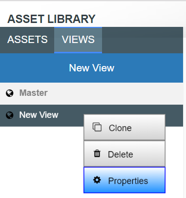
Metadata in Akumen is generally stored in grids, for example the Application Manager grid or the Pages grid. Each of these grids within Akumen has a right-click context menu that provides additional functionality, such as deleting, cloning or even viewing the properties of the selected item.
The Asset Library allows you to store data about your business.
To address the problem of data consistency and integrity, Akumen encourages the use of an Asset Library. The Asset Library acts as a single source of truth. It is a staging area for all the fixed values across the business.
An Asset is any “concept” in the business. These could be physical assets like infrastructure or equipment, or intangible assets like bank accounts, loans or rent.
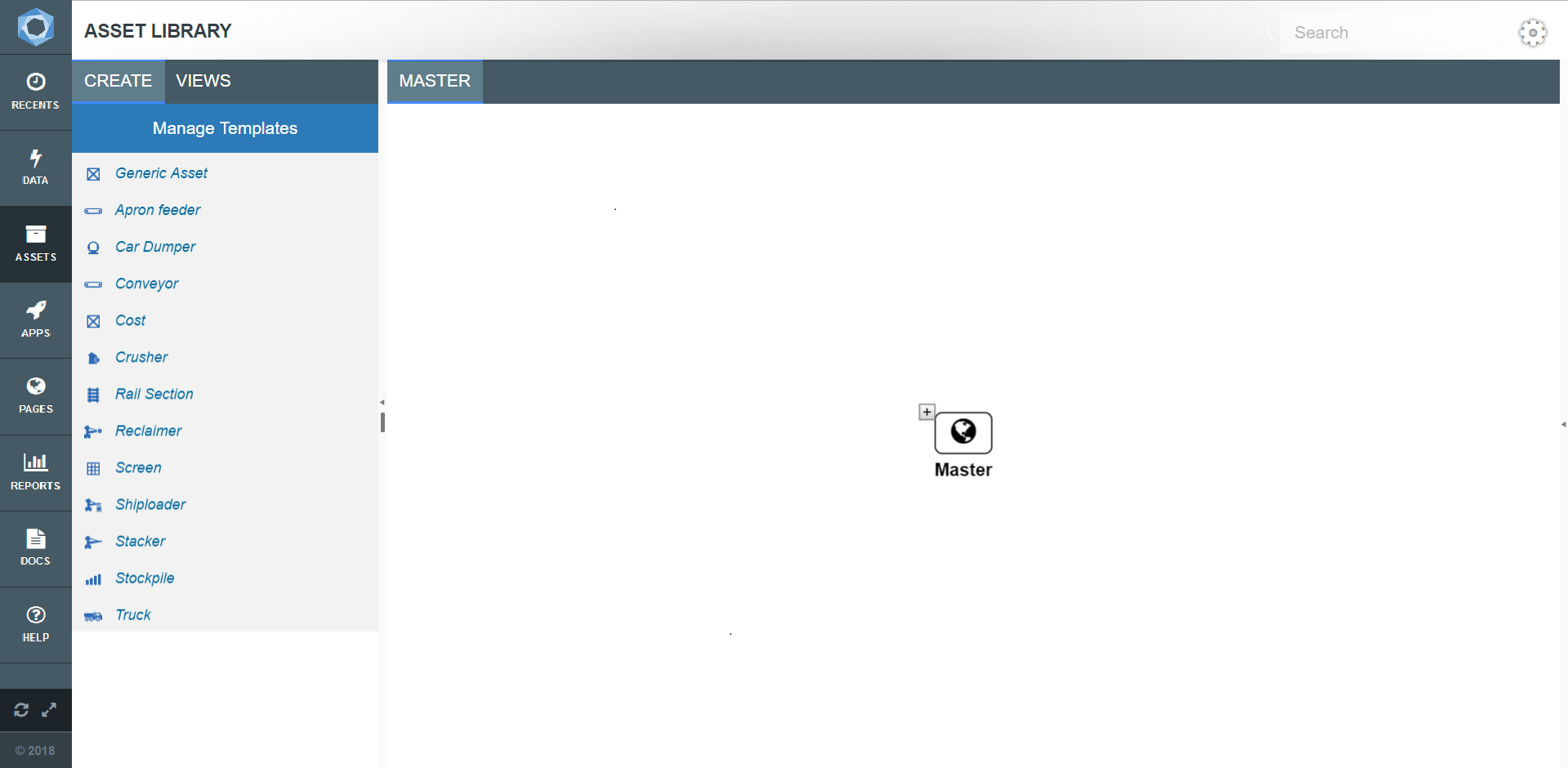
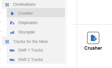
There are two main areas of the Asset Library as seen in the image below.
Asset templates provide a way of setting up the attributes of a template once. Every time that template is used to create a new asset, the attributes are automatically created with that asset. For example, creating an asset of type Crusher will include attributes such as: Name Plate Rate and Manufacturer.
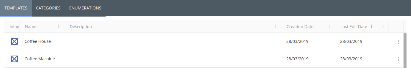
They are accessible through the Manage Templates button in the Create tab in the Asset Library, or through the Cog, Configure, Asset Templates.
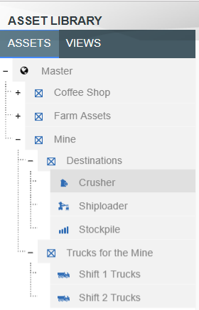
The Master View is where all of the fixed data for your applications are stored in a hierarchical format.
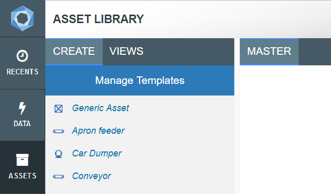
We’ve seen that the left pane has two tabs one of which is Create. The Create tab allows users to create assets based on templates.
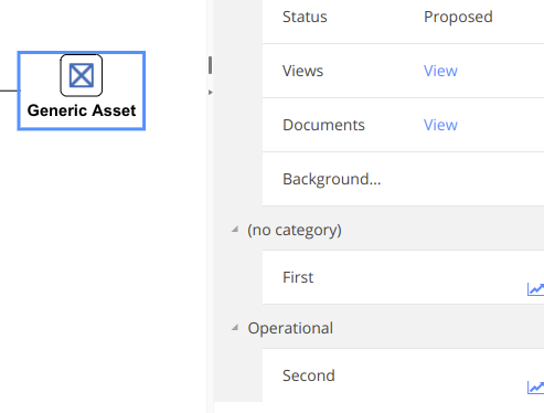
By dragging a template onto the Master View icon, users can attach an Asset to the Master View. If an asset template is dragged onto another asset than that asset becomes part of that branch.
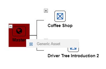
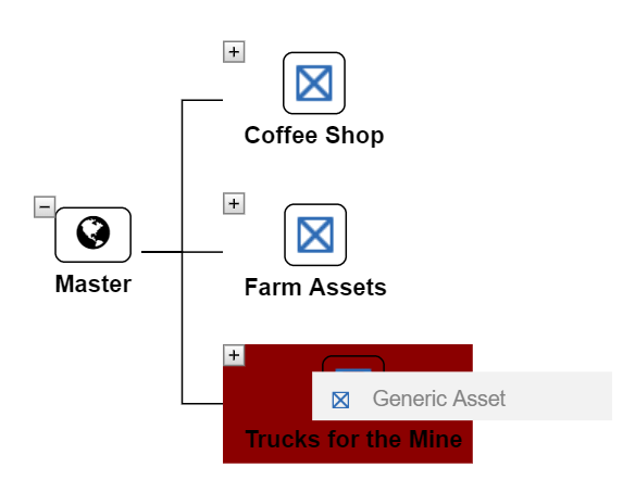
To add an Asset to the Master view:
Each Asset must have a unique name so that they can be linked to from within applications.
Every Asset template has a set of properties attached to it. For example a truck asset will have a specific set of properties attached to it which will differ from those of a cost or conveyor asset.
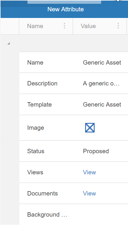
Each template has a selection of data points surrounding each Asset. These are called attributes. These attributes are only suggestions and each point does not need to be filled in for models to run. Models that do draw information from the Asset Library will only take the asset information available to it.
If a model is run that does require specific information from the Asset Library and it does not exist within the Asset, the model will leave that piece of information blank. If the information is required by the model an error will be returned when the model is run asking users to enter the required information.
However, templates do not always have all the needed attributes for a particular Asset. Sometimes Attributes will have to be created in order to add extra information regarding the Asset. These can be added by simply hitting the “New Attribute” button in the configuration pane of a selected asset. Once an attribute has been created, either through the template or manually through the asset, selecting the asset will bring up a properties pane allowing the user to edit the value.
If no value is set for an attribute then that attribute will not appear in the Driver Model asset parameter node menu.
There are several default categories available - each attribute must be allocated to one category:
New categories can be added in the Asset Templates screen, under the “Categories” tab.
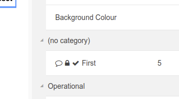
When a new attribute is created it will appear under the appropriate category in the configuration pane of a selected asset
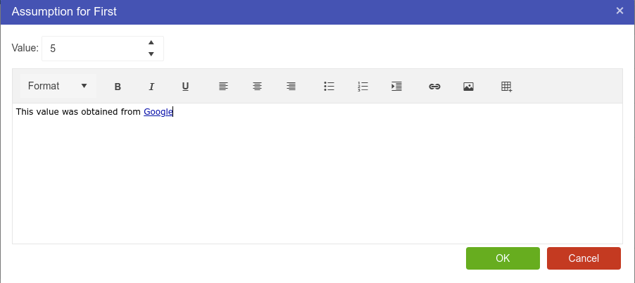
Any asset attribute can have an assumption entered against that attribute. Simply Right Click the attribute, and hit the Assumptions button. A popup window will appear allow you to enter some rich text about the attribute.
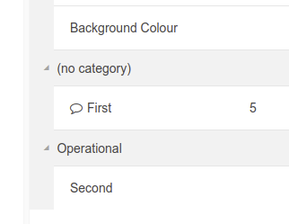
Once the record is saved, a comment icon will appear next to the attribute in the properties grid.
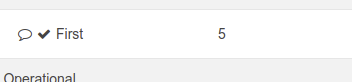
Attributes can be marked as approved by right clicking and hitting the approve button. Once approved, a check icon appears next to the attribute, as well as a tooltip indicating the approver’s details. To remove the approval, simply alter the value.
Attributes can also be locked such that they cannot be edited. Similar to approvals, right click an attribute to lock it. A padlock will appear next to the attribute, and prevent editing. Note that this is different from security, as attributes can also be unlocked by right clicking.
The primary use case for this functionality is if you have a model that calculates an asset value, or populates it from an external source, you do not generally want users modifying this value. An API call can lock the parameter, but it also does not adhere to the same restrictions the user interface has in regards to locking (ie the value can be edited programmatically, just not through the user interface).
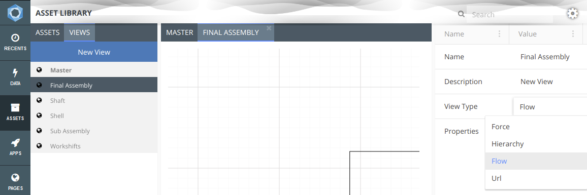
There are a number of different types of views. Each view allows users to see assets from the Master view in different ways:
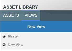
To create a New View select New View at the top of the left pane in the views tab. A new view will automatically be created.
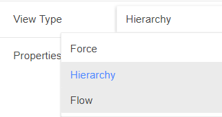
To change the type of view:
In the properties panel of the View you can also change the view’s:
We recommend giving each view a specific and unique name so that it can be easily identified from other views.
There are four types of Views you can create:
This view is exactly like your original Master View. The Master View shows all of the Assets in the Asset Library in the form of a hierarchy tree. Although similar to the Master View, the hierarchy view allows users to choose specific branches of the Master Tree they want to view. This is especially useful when setting up permissions as part of our recommended Best Practices for Akumen.
Hierarchy Views isolate user defined branches and when users select that view they will only be able to see that particular branch.
To create a Hierarchy View:
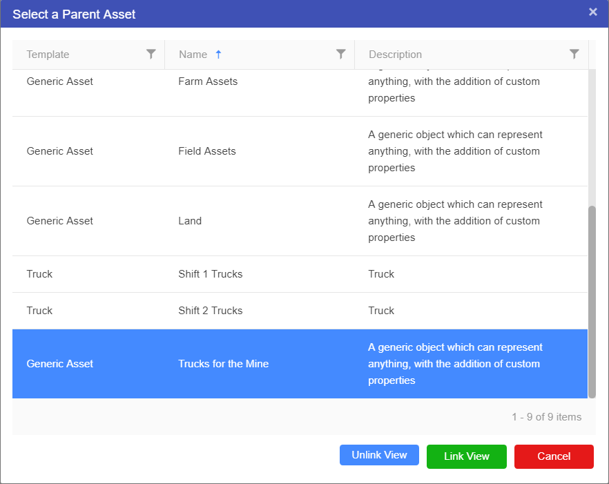
Hierarchy Views can be created from scratch by dragging and dropping assets from the Assets palette on the left of screen, or an asset can be set as a parent, in effect linking the current view to a section of the Master View.
To link a view to an asset in the Master view:

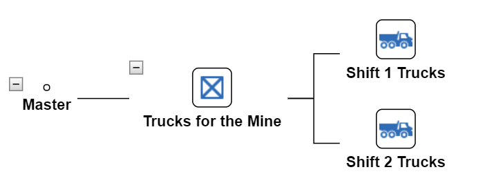
Is a way of representing data in the form of a network, similar to a mind map.
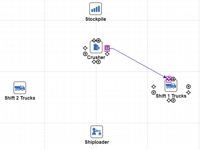
A Flow View allows users to create a flow diagram linking assets together. This is most useful when trying to model supply chains or logistics flows. Unlike Hierarchy Views Flow views are not linked on one specific asset of a branch. Users can draw on assets from all over the Master Tree to create their flow.
To create a Flow View:
You can create an application by using code based Python or R models, or graphical Driver Models.
Build your model once and use it to perform multiple what-if scenarios.
Value Driver Models (VDMs) allow subject-matter experts to build graphical models, and easily share them throughout your organisation.
Before we launch into Driver Models, what different nodes do and how to connect them to each other, it is important to understand the very basics of a Driver Model.
For this manual we will be using different examples to explain each node. It is recommended that you create multiple Applications so that you can experiment with the Driver Models described in this manual, expand on them, or even use them to create something entirely different.
A Driver Model graphically represents inputs and equations in a free form tree diagram allowing users to determine the key factors that impact results.
Akumen Driver Models are based on Value Driver Models – a technique commonly used in Business and Process Improvement.
To create a new Driver Model:

There are few extra things to note about the creation of Applications in Akumen. The first is that if you leave your application at any time you can always get back to it by either going through the Application Manager or the RECENTS tab. Both will take you straight back to your Driver Model.
If you are looking at the Application Manager you will also notice how there is an icon that has three vertical dots at the right end of each App.

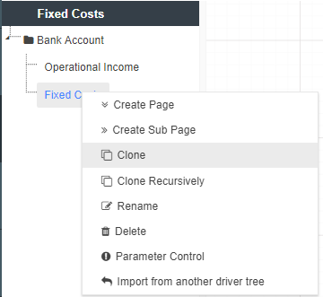
If you click on the above icon (or simply right click the application) the following options will be brought up:
All of the above options make it possible for you to modify your model’s properties, attach important information to your model, and create new versions of your model if needed.
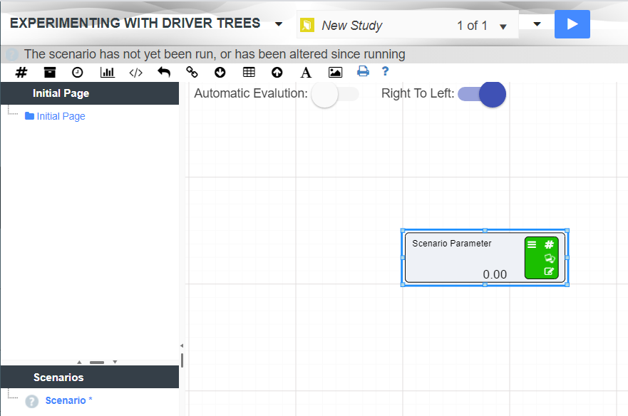
Once you have created your new Driver Model App, you will be taken to the main Driver Model page. The main page looks like the image below.
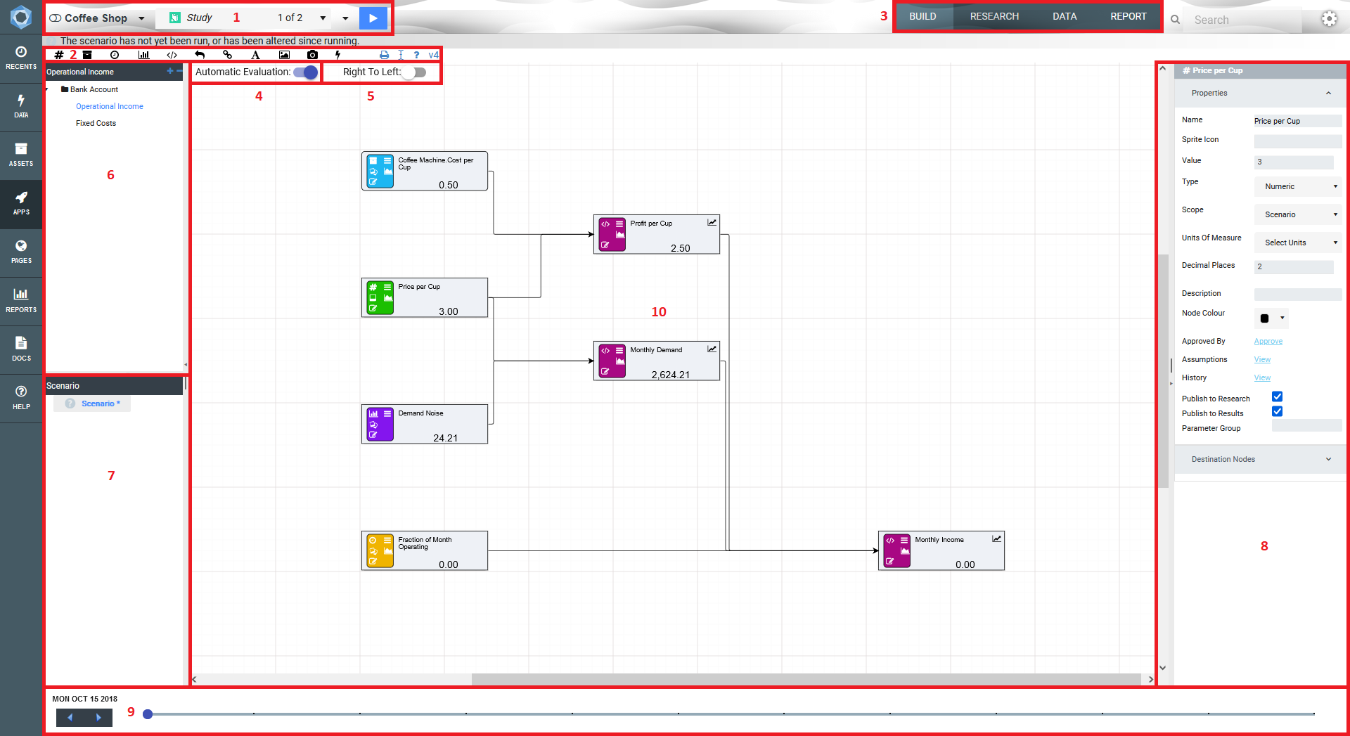
There are ten main areas for a driver model:
In the Driver Model Editor we pointed out the ten major areas of the editor. Number 5 allows users to decide what style of Driver Model they would like to create.
There are two options:
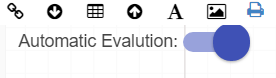
Both are able to be selected by clicking on the Right to Left switch at top left of the editor, next to the Automatic Evaluation switch and under the Node Palette.
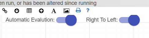
By default, the style of the Driver Model is set to Right to Left.
Setting the Driver Model direction depends on the type of Driver Model you want to create.
Right to Left is for traditional driver models, such as those used in Lean.
Left to Right is more commonly associated with process flows and schematic type layouts.
Driver Model Pages allows driver models to be broken up into different areas. Although smaller driver models can easily be accomodated in a single page, breaking the driver model up into multiple pages makes it much easier to understand the driver model. Examples of breaking driver models into pages include things like processing areas or even different business areas. Continue driver model evaluations from one page to the next is handled through
There are several different ways to create a new Page. We can:
When a page is cloned, the source page and all it’s nodes are copied (the nodes are clones of the originals, not the actual originals - Akumen will automatically rename all the node names to ensure there are no clashing node names). Once cloned you can treat the new driver model page as a new page, meaning you can:
Whatever changes you make to the cloned page do not effect the parent page.
When creating new pages they can either be created on the same level as the parent page or as a subpage of the parent page. Creating a new subpage gives you a blank workspace to start with and visually links the new subpage with the parent page.
Recursive Cloning clones the selected Driver Model page and all of its children pages creating an entirely new version of your Driver Model.
We provide the option to export data from a driver model to Excel. Only scenarios that have been executed will appear in the exported Excel document.
There are three ways to perform an export of VDM scenario data to Excel:
Model: Exports all studies and their associated scenarios to Excel. Only exported scenarios will appear in the Excel document.
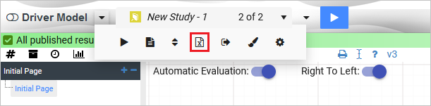
Study: Exports an individual study and its associated scenarios to Excel. Only exported scenarios will appear in the Excel document.
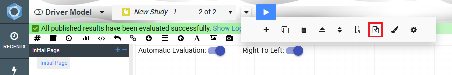
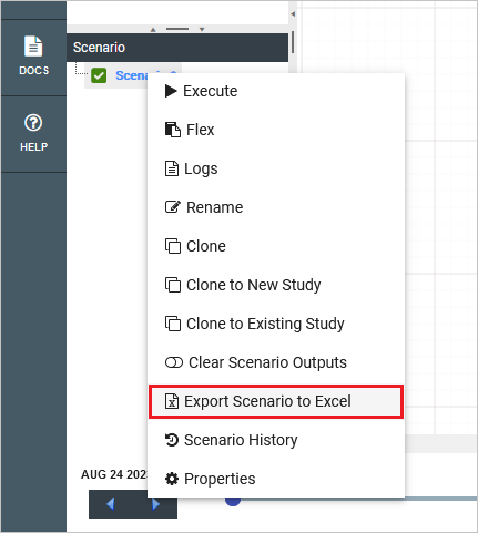
Scenario: Exports an individual scenario to Excel. This is performed by right-clicking the scenario and selecting Export Scenario to Excel.
Note that this option will only appear if the scenario has been executed.
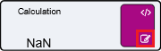
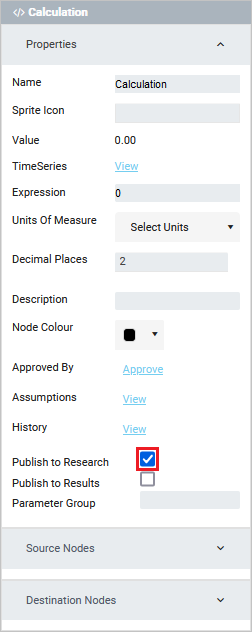
Calculation nodes do not appear in the exported Excel document by default. For these nodes to appear, they need to first be published to the research grid. This can be done as follows:
Properties for the calculation node as shown in the image below.
Publish to Research has been ticked.
There are many different node types that will aid you in building your Driver Model.
These node types are:
Now that we have covered the basics of driver models we are ready to begin understanding the different nodes, how to connect them to create flows and build models and systems.
To do this we will use very simple examples which demonstrate a node’s capabilities.
A parameter group is used to arrange node results into named output tables. By default, node values that are published to results will appear in the “appoutput_vw” table. By specifying a parameter group, these node values can be added into either a single or multiple output tables.
Parameter group names are added to multiple output tables separated using a comma delimiter. For example, a node could be added to parameter groups “test1” and “test2” by specifying “test1,test2” in the node’s paramater groups field.
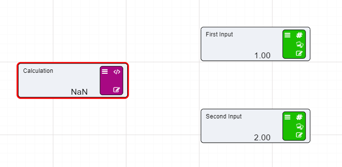
There are many different node types that can be used to create Driver Models. The simplest of these nodes is the Numeric node. Numeric nodes hold onto values to be used in the application. They are placeholder nodes. They are assigned values that will not be used until they are attached to a:
They are also excellent at demonstrating how to edit, connect, and use nodes to create a Driver Model.
To show you how to use a Numeric node we will set up two numeric nodes in preparation for the following slide on Calculation nodes.
To set up a Numeric nodes:

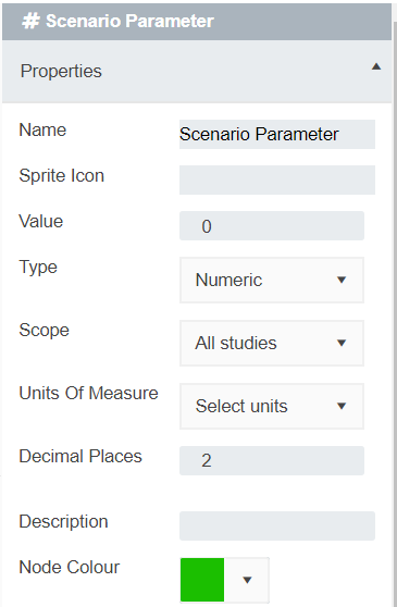
You probably noticed that in the editing window of the Numeric node you could set:
All of these things can be changed in a Numeric node. For example, if we were going to set a value of $50, we would just have to set the units of measure to $ and make sure that the number of decimal places visible was set to 2.
This list in the editing window is the same for the following nodes:
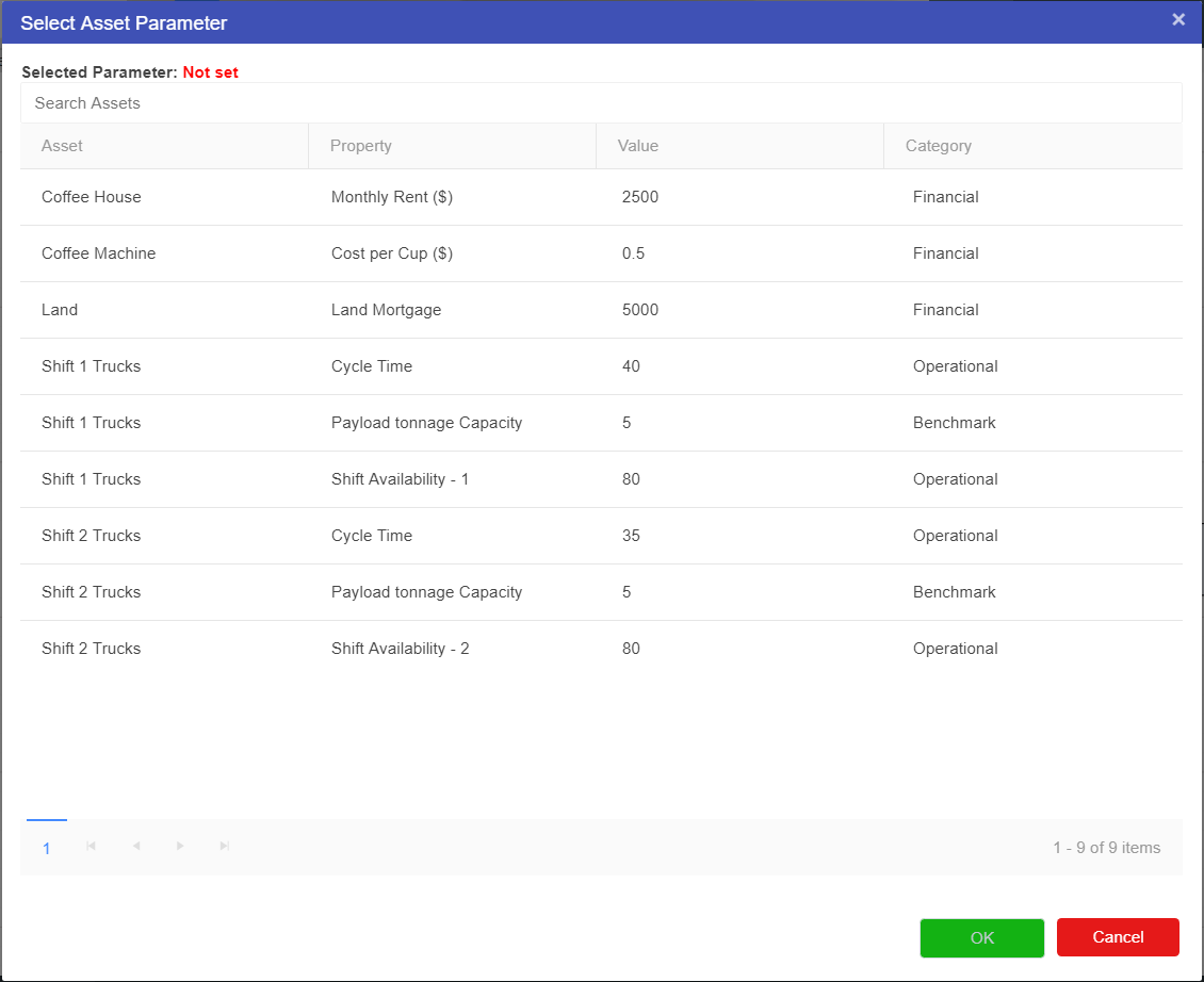
The Asset Parameter node is the connection between the Asset Library and Driver Models. By using an Asset Parameter node users can get values stored in the Asset Library and bring them into the Driver Model. Since Asset values cannot be changed outside the Asset Library these values will remain the same during scenario analysis.
Click here to learn more about the Asset Library.
To set up an Asset Parameter node we should first have an Asset to link to the node. Once you have this Asset you can link it to the Asset Parameter node.
To do this:
 onto the workspace.
The Asset Parameter node will appear blank (see screenshot below) until an Asset is selected.
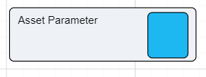
You now have an Asset Parameter node.
Although asset parameter nodes cannot be changed from the driver model, they can be converted into Scenario Input parameters to see the effects of changing the value throughout the model. The best practice for this is to leave the asset parameter as is in the “base” scenario, then cloning the scenario and converting the node to a numeric, as shown in Changing Node Types.
Remember you cannot edit an Asset value outside of the Asset Library. If you do wish to edit the value of an Asset you will have to go to the Asset Library. Editing the value in the Asset Library will change the value for every model using this value.
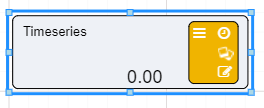
These nodes allow models to predict outcome values for the model over time. They allow users to define a time period and assign values for each of those time periods. The timeseries node will need to be connected to a Calculation node before the values in the timeseries node will affect the Driver Model.
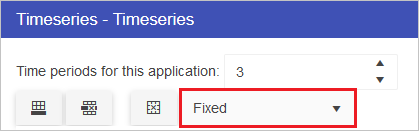
Prior to creating any timeseries nodes, the number of periods and reporting period (below) as well as the start date, can be defined by changing the model properties. In addition, it is sometimes desirable (especially in finance VDMs), to have different scenarios represent different time periods. This can be done by setting the Start Date in the scenario properties.
When setting up a timeseries node, users can define:
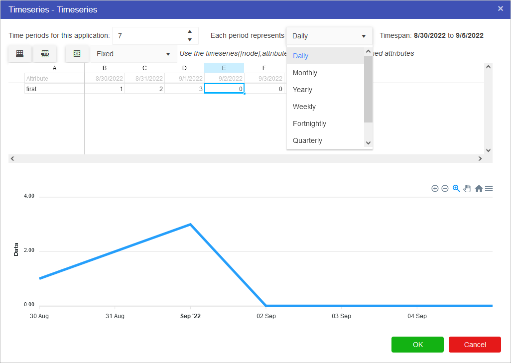
If we, for example, wanted to look at the the value of gold over the course of the week we would put in:
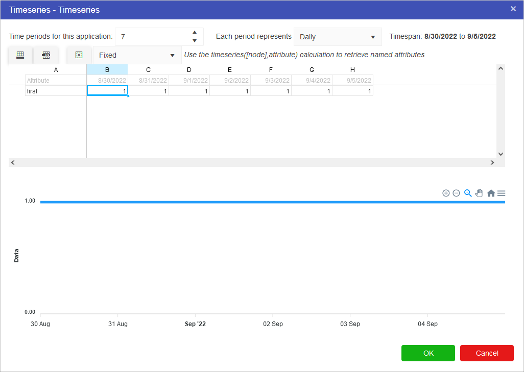
Note that the values specified for the number of periods and period type will affect the entire model. If you had two timeseries nodes on the page, altering the number of time periods would affect both nodes. This setting is also available in the model properties.
If we knew that the value fluctuated throughout the week between 50% of the value at the start of the week and 100% then we could plan for the worst case and the best case by using scenarios and in the second scenario we could change the timeseries values to 0.5 for 50%.
To set up a Timeseries node:
 onto the workspace.
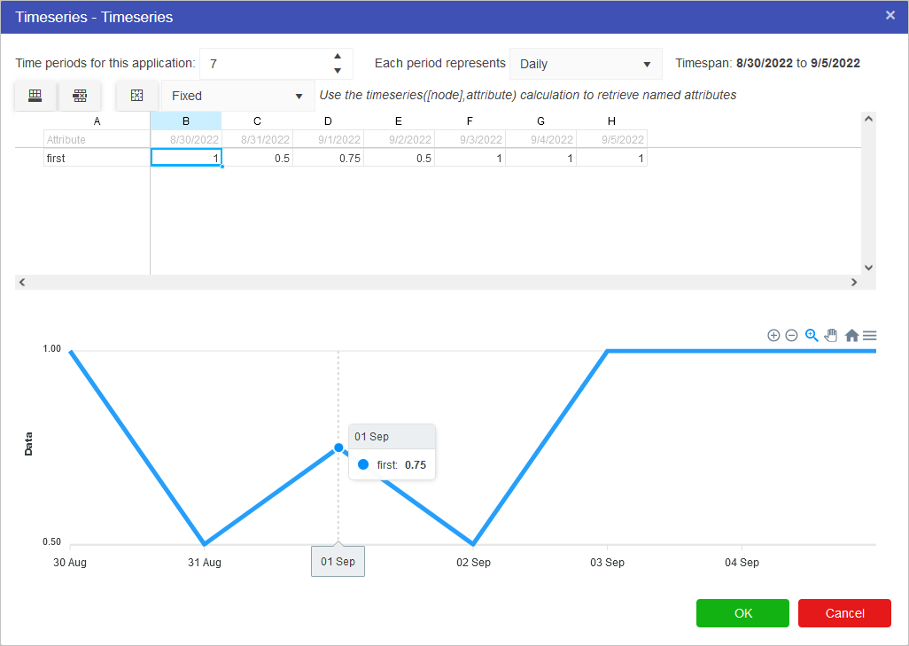
Whenever a new Timeseries node is added to the Driver Model, a slider will appear at the bottom of the screen. The number of periods displayed in the timeslider are the number of periods specified in the timeseries node OR the model properties. To see the effects over time, simply slide the bar to the next time interval.

Multiple different timeseries sets can be defined per timeseries node. The buttons highlight below control this functionality. From left to right, these options are:
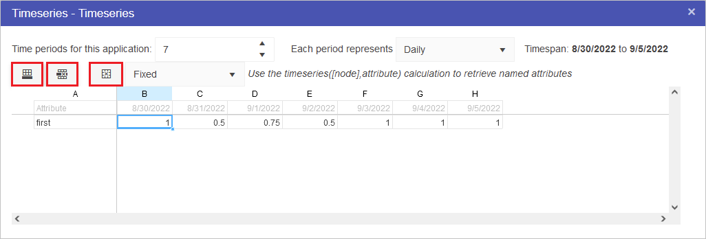
The dropdown menu contains options for Fixed, Interpolate and Last Known Value. These work as follows:
The last day of the month will always be selected if the period increment is set to “Monthly” or “Quarterly” and the model start date is set to the last day of the month. For example, if the model start date is set to 28-Feb-2022 on a quarterly increment, the next period will be 31-May-2022 instead of 28-May-2022.
Calculation nodes are probably the most important node in a Driver Model. They take inputs from the different nodes and use their values in mathematical expressions to produce an output value.
Calculation nodes do not need to have inputs to work. Expressions and values without the input of the other nodes can be entered into a Calculation node to produce a value. However, anytime you wish to change that value you will need to go into the expression editor within the Calculation node and manually change the value. This is why we recommend that for any expression entered into a Calculation node there is always a node which holds the input value so that:
On the previous page we set up two Numeric nodes in a Driver Model workspace. We will now demonstrate how the Calculation nodes work by using the previously created Numeric nodes and putting them into an Expression in a Calculation node.
To set up a Calculation node:
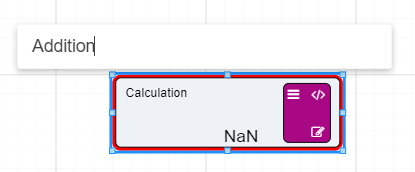
Change the name of the Calculation node by clicking on the current name of the node and waiting for an editing bar to appear above the node.
This is how you would change the name of a node without going into the editing bar.
Note
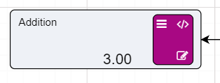
Rename your Calculation node to Addition.
Now that we have set up our Calculation node we will need to add the inputs to the Calculation node.
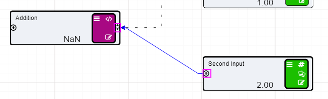
You will notice that the two Numeric nodes are now connected to the Calculation node by dotted lines. These lines mean that the inputs are connected to the Calculation node but they are not being used in the expression. The lines will become solid once we add these values to our expression.
Expressions in Calculation node are written in a similar format to that of an Excel expression.
To get a result from the Calculation node we have to set up an expression. To set up an expression:
 For this example we will add the two Numeric nodes together, but more complex expressions can be written in the expression editor.
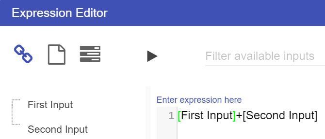
Notice that the dotted lines between the nodes will now be solid as the values of those nodes are now in use.
References to nodes in the Expression Editor must surround the node name with [ ]
When Calculation nodes are given inputs, they become dependent on those nodes. So, if for example our First Input Node was to change from 1 to 5 the calculated value would become 7. And if the Second Input was to change from 2 to 6 then calculated value would become 11.
Calculation nodes do not have to remain the same in terms of expression. Expressions can change at any time. Should the expression change from Addition to subtraction all users would need to do would be to go into the expression editor and change the “+” to a “-”. This would result in the value going from 11 to 1. If we wanted to divide 5 by 6 we would put a “/” in between the First Input Node and the Second Input Node. And if we wanted to multiply the two nodes, we would adjust the symbol from a “/” to a “*”.
There is no limit on the amount of inputs, however some functions do have a limited number of inputs. They do have to be put into the expression though before their values will be used by the node.
Code comments can be used in calculations using // syntax.
The below tables list the functions and operators available for Driver Models.
| Type | Operator | Notes |
|---|---|---|
| Arithmetic | + - * / | The standard arithmetic operators |
| Arithmetic | % | modulus, or remainder |
| Arithmetic | ^ ** | “to the power of”. x^y can be written as x**y or pow(x,y) |
| Logical Boolean | && || ! | And, Or, Not |
| Bitwise | & | xor | And, Or, Xor |
| Comparison | > < >= <= | Greater than, Less Than, Greater Than or Equal To, Less Than or Equal To |
| Comparison | = == | Is Equal To |
| Comparison | != | Is Not Equal To |
| Constants | e pi | Euler’s constant, approximately 2.7182818, Pi, approximately 3.14159265 |
| Function | Notes |
|---|---|
abs(Number) |
Returns the absolute value of the specified number |
acos(Number) |
Returns the angle whose cosine is the specified number |
asin(Number) |
Returns the angle whose sine is the specified number |
atan(Number) |
Returns the angle whose tangent is the specified number |
ceiling(Number) |
Returns the smallest integral value that is greater than or equal to the specified number |
cos(Angle) |
Returns the cosine of the given angle |
cosh(Angle) |
Returns the hyperbolic cosine of the specified angle |
exp(Number) |
Returns e raised to the specified power |
floor(Number) |
Returns the largest integer less than or equal to the specified number |
ln(Number) |
Returns the natural (base e) logarithm of a number |
log10(Number) |
Returns the natural (base 10) logarithm of a number |
log(Number, Base) |
Returns the logarithm of a number in a specified base |
pow(Number, Power) |
Returns a number raised to the specified power |
rand() |
Returns a random number between 0 and 1 |
rangepart(value, min[, max]) |
Returns that part of a value that lies between min and max) |
round(Number[, d]) |
Rounds the argument, (optionally to the nearest ’d’ decimal places) |
sin(Angle) |
Returns the sine of the given angle |
sinh(Angle) |
Returns the hyperbolic sine of the specified angle |
sqrt(Number) |
Returns the square root of the specified number |
tan(Angle) |
Returns the tangent of the given angle |
tanh(Angle) |
Returns the hyperbolic tangent of the specified angle |
trunc(Number) |
Rounds the specified number to the nearest integer towards zero |
| Function | Notes |
|---|---|
avg(A, B, C, ..n) |
Returns the average of the specified numbers |
max(A, B, C, ..n) |
Returns the maximum of the specified numbers |
min(A, B, C, ..n) |
Returns the minimum of the specified numbers |
sum(A, B, C, ..n) |
Returns the sum of the specified numbers |
| Function | Notes |
|---|---|
asset(AssetName, AttributeName) |
Returns the value of an attribute on an asset |
simulationruntime() |
Returns the simulation time (from the active scenario) |
periodCurrent() |
Gets the current 0 based period number |
periodAverage(N[,[start][,end][,error_value]) |
Returns the cumulative average of the argument over all the model iterations to date, or between start and end if set. Error value applies prior to values prior to the range, or if not set the period 0 value |
periodWeightedAverage(N, W[,[start][,end][,error_value]) |
Returns the cumulative weighed average of the argument over all the model iterations to date, or between start and end if set. Error value applies prior to values prior to the range, or if not set the period 0 value |
periodCount([N,[start][,end]) |
Returns the number of model iterations to date, or between start and end if set. |
periodFirst(N) |
Returns the value of the argument at the first model iteration. |
periodLast(N) |
Returns the value of the argument at the last model iteration. |
periodMax(N[,start][,end][,error_value]) |
Returns the high-water-mark of the argument over all the model iterations to date, or between start and end if set. Error value applies prior to values prior to the range, or if not set the period 0 value |
periodMin(N[,start][,end][,error_value]) |
Returns the low-water-mark of the argument over all the model iterations to date, or between start and end if set. Error value applies prior to values prior to the range, or if not set the period 0 value |
periodSum(N[,start][,end][,error_value]) |
Returns the cumulative sum of the argument over all the model iterations to date, or between start and end if set. Error value applies prior to values prior to the range, or if not set the period 0 value |
periodOpeningBalance(I[,A[,R]]) |
Returns the start-of-period balance, based on an Initial balance and accruing Additions and Removals on each subsequent period. |
periodClosingBalance(I[,A[,R]]) |
Returns the end-of-period balance, based on an Initial balance and accruing Additions and Removals on each period. |
periodPresentValue(d, N) |
Returns the present value of parameter N using the specified discount rate of d |
periodNPV(d, N) |
Returns the NPV of parameter N using the specified discount rate of d |
periodDelay(p, N[, default]) |
Returns the value of the argument N, but p periods later. Prior to that, it returns optional [default], else 0 |
periodVar(N) |
Returns the variance of the argument N |
relativePeriodSum([node], N) |
Returns the period sum of “node” over a rolling window into the past. The value of “N” determines the number of periods to go into the past including the current period. |
| Function | Notes |
|---|---|
periodAverageAll(N) |
Returns the average of the argument over all of the time periods |
periodCountAll() |
Returns the total number of periods |
periodLastAll(N) |
Returns the value of the argument in the last period |
periodMaxAll(N) |
Returns the maximum value of the argument over all of the time periods |
periodMinAll(N) |
Returns the minimum value of the argument over all of the time periods |
periodSumAll(N) |
Returns the sum value of the argument over all of the time periods |
periodWeightedAverageAll(N, W) |
Returns the weighted average of the argument N over all of the time periods, weighted by W |
| Function | Notes |
|---|---|
if(test,truepart,falsepart) |
If ’test’ is true, returns ’truepart’, else ‘falsepart’ |
iferror(calculation, errorresult) |
If ‘calculation’ has an error, return the error result, otherwise return the result of ‘calculation’ |
switch(value, condition, result, condition2, result2, condition3, result3, ...) |
Evaluates a value, then returns the result associated with the value |
| Function | Notes |
|---|---|
AverageIf(condition, N) |
Returns the cumulative average of the argument over all the model iterations to date if the condition is met |
CountIf(condition) |
Returns the number of model iterations to date if the condition is met |
SumIf(condition, N) |
Returns the cumulative sum of the argument over all the model iterations to date if the condition is met |
| Function | Notes |
|---|---|
execute(model name, period, input1Name, [input1Node], input2Name, [input2Node], ...) |
Executes an Akumen app (use period for the period number in driver models, 0 for Py/R). Returns 0 if successfull, otherwise -1. Note that this is not intended for large Py/R models, and could cause a performance impact. It is designed to be used as simple helper functions the driver model cannot perform. It is also limited to int/float inputs only |
executeoutput([executeNode], output1Name) |
Returns the result of the execute function, getting the value output1Name from the result. This is limited to simple int/float outputs only |
See here for information on setting up datasources, or here for further information on how to use datasources within Value Driver Models.
| Function | Notes |
|---|---|
datasource([datasource_node], value_column, aggregation_method, forwardfill, forwardfillstartingvalue, filter1column, filter1value, filter2column, filter2value, ...) |
Links a calculation to the datasource and applies an optional filter |
datasourceall([datasource_node], value_column, aggregation_method, forwardfill, forwardfillstartingvalue, filter1column, filter1value, filter2column, filter2value, ...) |
Links a calculation to the datasource and applies an optional filter |
Datasource specific filtering can be used across multiple columns in the datasource by adding in filter2column, filter2value, filter3column, filter3value etc.
datasourceall can also be used in place of datasource (using the same parameters). Instead of operating at a single time period, it operates across the entire dataset (honouring the load id and additional filter). This allows you to do things like get the stddev or mean of the entire dataset.
If only one row exists in the timeseries node, data can be referenced in the calculation formula by only providing the timeseries node name.
If multiple rows exist, the row name will need to be specified in the calculation formula as well. See grid below for calculation formula formats.
| Function | Notes |
|---|---|
timeseries([timeseries_node]) |
References time series node with name “timeseries_node” |
timeseries(timeseries([timeseries_node],"row_name")) |
References time series node with name “timeseries_node” and row label “row_name” |
timeseries([timeseries_node],[numeric_node_name]) |
References time series node with name “timeseries_node” and the row set to the 0-based value “numeric_node_name” |
| Function | Notes |
|---|---|
CurrentDayInMonth() |
The numerical day of the month of the current period |
CurrentDayInWeek() |
The numerical day of the week of the current period |
CurrentDayInYear() |
The numerical day of the year of the current period |
CurrentMonth() |
The numerical current month |
CurrentPeriodDateTimeUtc() |
The current period datetime in Excel format (ie 40000) |
CurrentYear() |
The numerical current year |
DaysInMonth() |
The numerical days in the month |
FirstPeriodDateTimeUtc() |
Period 0’s datetime in Excel format |
LastPeriodDateTimeUtc() |
The last period’s datetime in Excel format |
NumPeriods() |
The number of periods in the model |
| Function |
|---|
ContinuousUniform(lower, upper, [seed]) |
Lognormal(mu, signma, [seed]) |
Normal(mean, stddev, [seed]) |
Pert(min, mostlikely, max, [seed]) |
Triangular(lower, upper, mode, [seed]) |
The seed is optional, and applies at time period 0. This means that the random number generated for time period 0 will always be the same as long as the seed remains the same. The following periods reuse the random number generator meaning the pattern of numbers will be exactly the same for each execution. This guarantees consistency of results. The seed can also be applied using a scenario parameter.
Click here for more information on range checking nodes.
| Function | Notes |
|---|---|
rangecheck(sourcenode, lowlow, low, high, highhigh) |
Performs a check against of the source nodes value against the limits |
rangecheckresult(rangechecknode) |
Returns a value corresponding to which limit has been broken. -2 = lowlow, -1 = low, 0 = none, 1 = high, 2 = highhigh |
Node groups (nodegroup(), nodeungroup()) are used to collapse multiple nodes into a group that can be used in different areas.
For example, you can collapse a group of nodes and feed it into a Component. Once inside the component, the node group can be ungrouped to get the individual nodes within the component.
Node groups can also be processed into arrays. A node group will become a column in an array, with the name of the column being _NodeGroupName (note the underscore).
The underscore is there to distinguish between the node and the column (when array based functions are used),
with the names of the array rows being the inputs that make up the node group. Note that the names of the rows can be changed with the arraysetrownames() function.
There is no need for the nodeungroup() calc when using arrays as the node group is already ungrouped into the array.
Multiple node groups can be used to quickly build arrays, but they must all be the same length.
Component functions allow groups of nodes to be created as reusable components, rather than copying and pasting the nodes. These are similar to functions in normal programming.
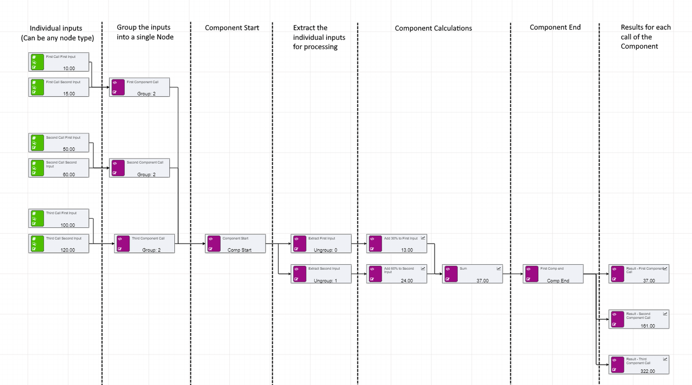
See image below for an example.
In this example, a reusable component has been created between the Component Start and Component End nodes. The start and end nodes define the boundary of the component.
The Component Start node can only receive incoming data from a nodegroup node, which combines the incoming nodes into a single feed.
Once inside the component, the nodeungroup() function allows the modeller to split the node group into individual entries.
The overall component will run once per node group. So in this example, the component will run twice.
The nodes feeding into the component end can be retrieved using a componentresult() function.
| Dynamic | Function | Notes |
|---|---|---|
| x | componentstart() |
This is the main entry point to the component. Only nodegroups can be connected to the component start. It is possible to add another component start within an existing component but this may create unforseen issues and errors and therefore only one componentstart/component end should be used.This only supports dynamically linked nodes. It is not necessary to type in the names of the node group node. |
| x | componentend([componentstart]) |
The componentend calculation indicates the end point of the component. Every input to the component runs once between the componentstart and componentend. This only supports dynamically linked nodes. Only the componentstart node is required. |
componentresult([componentend], run_index, "calculated_node") |
This calculation fetches the result for the selected run index. The run index is the index of the node group that is passed into component start, as they are ordered on the driver model canvas - first by the y-axis, then by the x-axis.If there are multiple calculated values to fetch, then the calculated node can be optionally added. If the calculated node is not included in the expression, it defaults to the first calculated node connected to componentend.The run_index can be a fixed number referencing the index (x, y ordered) of the run, or the name of the node group that feeds into the componentstart. Note that the name of the node group should be double quoted, rather than enclosed in square brackets. | |
| x | nodegroup() |
Groups a set of nodes for use in calculations, such as components or arrays |
| x | nodeungroup(index, [componentstart]) |
Gets the node based on the index for use in calculations. |
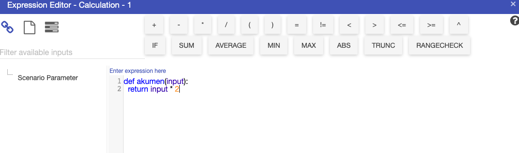
Python nodes allow individual driver model nodes to include Python code directly in the node calculation as shown in the example below.
The number of inputs being linked into the Python (calculation) node must exactly match the number of parameters defined by the Python function, this is not dynamic.
Like dynamic nodes, however, the order of the nodes fed in matters. This is determined by positions of the nodes on the driver model canvas - first by the y-axis, then by the x-axis.
Also the names in the def akumen(…) or def runonce(…) function are NOT the names of the nodes. They are instead Python variables and therefore cannot have special characters or spaces in the names.
The value of the incoming node will come through as the variable’s value.
To create a Python function, the first line must be either of the following:
def akumen(input1, input2):def runonce(input1, input2):The syntax highlighting will automatically convert to Python highlighting. The akumen() function will run for every time period and is limited to a 1 second runtime.
The runonce() function will run for time period 0 only and cache the result. This result is then passed into every other time period.
It is limited to a 5 second runtime and can be used for data preparation tasks (e.g. retrieving output from a datasource, cleaning the data and then passing the output to a datasource calculation.
All Python nodes need a return statement which is used to output the results of the Python code to other nodes.
If there is a single scalar value in the return, it can be referenced directly within any other calculation.
There is also the option to return a dictionary of values.
These cannot be referenced directly and require the pythonresult() function (e.g. pythonresult([python_node], "first")) which will allow access to the dictionary values.
This allows the Python node to return multiple values in one function and is more efficient than using multiple Python nodes with similar code, as the code is only executed once.
There are some limitations with Python nodes:
In addition to the list associated above, a subset of Pandas functions are available as aliases. The full Pandas module cannot be imported directly due to security concerns with some of the IO functionality Pandas provides.
The following Pandas functionality is available as aliases (note they are the exact pandas functions, only prefixed with pd_):
The following helpers provide additional quality of life improvements to the Python node:
array_helper - provides helper functions for dealing with arrays out of the calc engine:
| Function | Notes |
|---|---|
array_helper.convert_dataframe_to_array(datasource, columns, category_column) |
Converts a dataframe object (from a datasource) into an array. The value set for of “columns” is the list of columns to use, and “category_column” is the optional column to use as the category. If the first column is not a number, it automatically becomes the category column. If there is no category column in the list of columns, the index of the dataframe is used as the name. |
array_helper.convert_array_to_dataframe(array) |
Converts an array into a dataframe. |
period_helper - provides helper functions for dealing with periods in the calc engine:
| Function | Notes |
|---|---|
period_helper.get_current_period() |
Gets the period that the calc engine is currently on |
period_helper.get_reporting_period() |
Gets the reporting period that is configured |
period_helper.get_num_periods() |
Gets the total number of detected periods |
period_helper.get_start_date() |
Gets the actual start date |
period_helper.get_date_from_period(period) |
Gets the date that corresponds to the selected period |
period_helper.get_period_from_date(date) |
Gets the period the period that corresponds to the date |
period_helper.convert_datetime_to_excel_serial_date(date) |
Converts the date to an excel serial date |
period_helper.convert_period_to_excel_serial_date(period) |
Converts the period to an excel date |
If preferred, alternative aliases can be used to reference the helper functions:
arrayhelper = ah (eg ah.convert_dataframe_to_array)periodhelper = ph (eg ph.get_current_period())The benefits to using Python nodes are:
pythonresult([pythonnode]).
Note there are no parameters specified. If a dictionary is returned, the first item in the dictionary is returned.When returning a dictionary, the Python node only executes once for a time period, and the result dictionary is cached. This makes it efficient to return multiple values from the Python node as a dictionary, rather than using multiple Python nodes.
Print statements can be specified in Python code (e.g. outputting the contents of variables, data frames, etc). While the print output won’t appear in the user interface when using auto-evaluation, it will appear in the normal Akumen log after performing a model execution.
Arrays are a ground breaking new piece of functionality for driver models. They can be built in a number of ways, including dynamically, from Python output as well as from datasources. Once data has been put into arrays, there are a number of array calculations which can be used to perform bulk operations, such as aggregations like sums and averages or sorting. In addition, groups of nodes can be added to arrays to make a single row of values.
Note that clicking on the table icon at the top right of the array node pops up a window showing the individual array values.
Arrays can be built in a number of different ways. This can be:
array() function (e.g. array (1, 2, 3, 4));arrayrow() function to feed data into the array to make individual rows; ornodegroup() to feed into the array to make individual columns.There are three basic modes of creating an array row:
Fixed is where values are entered directly into the node such as arrayrow(’name’,1,2,3,4,5). If a name is not provided, the name of the node will be used for the entire row. The name must have at least one alpha character.
Specified is where nodes that form the array row are entered in the column order required (e.g. arrayrow('name',[node2], [node3], [node4], [node5], [node6])).
If a name is not provided, the name of the node will be used for the row. The name must have at least one alpha character
Note that Fixed and specified entries can be intermixed.
Dynamic does not list any values or nodes within the function but rather uses nodes that are linked to the arrayrow() node (e.g. arrayrow('name')).
The order of the elements within the row is determined by the x and y locations of the linked source nodes on the driver model canvas (top to bottom, left to right).
If a name is not provided, the name of the node will be used for the row. The name must have at least one alpha character.
See below for an example of a simple arrayrow feeding into an array.
The node table contains the following data:
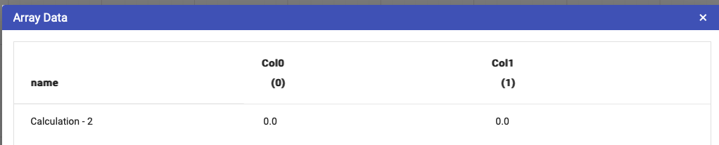
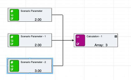
Node groups can also be used to build arrays. They are similar to arrayrows, but instead of building a row with multiple columns, the nodegroup becomes the column within the array. The row names become the node names from the first node group.
See below for an example of a simple nodegroup feeding into an array:
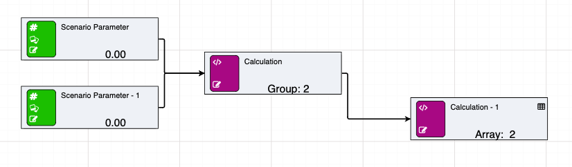
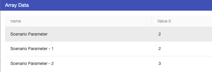
The node table contains the following data:
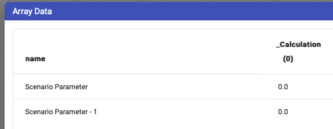
When passing a nodegroup into an array (or even individual input values), the node name is used as the column name. To distinguish between a node and a value, the calcengine prefixes an underscore (_) to the name of the column. This is done to allow calculated columns to identify the difference between a column and a node of the same name.
See table below for array functions.
| Dynamic | Function | Notes |
|---|---|---|
| Yes | array([input_1], [input_2], … [input_n]) |
Builds an array from either the supplied inputs, or dynamically from a datasource, another array (extending) or a Python node. Note if building from a Python node, then that must be the only input into the array. When building from a datasource, the datasource must be the first input (you cannot use dynamic) and the rest of the parameters are the names of the columns to bring in. Multiple columns will create rows of tuples see arraytuple(). Datasources no longer must have a date column specified. |
| Yes | arrayrow([input_1], [input_2], … [input_n]) |
Creates an array row, which is another way of saying a list of inputs. Array rows can be added to arrays, effectively forming a two dimension array. So for example, and array might be [2, 6, 3, 5], but an array of rows might be [(2, 4), (5, 6), (1, 2)]. This is useful when grouping like sets of data, such as height and weight for a person, or tonnes, iron, alumina, silica for a single product. Note that each row in the array must have the same number of columns. |
| No | arrayaverage([arraynode], column_index_or_name) |
Gets the average of the array, optionally providing the index of the column to aggregate. Not specifying the index assumes index = 0 |
| No | arraycount([arraynode]) |
Counts the number of items in the array |
| No | arraymatch([arraynode], [matchvalue], column_index_or_name, tolerance) |
Gets the index of the item matching the value. Setting approximate to true gets a close enough value, using the tolerance. When approximate and tolerance is set, the calculation used is: np.where(np.isclose(array_matches, match, atol=tolerance_value)) When just approximate is set, the calculation used is: np.where(np.isclose(array_matches, match)) When an exact match is used, the calculation used is: np.where(array_matches == match) |
| No | arrayfilter([arraynode], test_column, test, test_value) |
Filters an array (returning a new array) of the filtered items. This differs from match in that match will return a single index value, whereas filter returns a new array that is filtered based on a numeric condition. The syntax of the filter is:
|
| No | arraymin([arraynode], column_index_or_name) |
Gets the minimum value. Not specifying a column_index_or_name defaults to index = 0 |
| No | arraymax([arraynode], column_index_or_name) |
Gets the maximum value. Not specifying a column_index_or_name defaults to column_index_or_name = 0 |
| No | arraypercentile([arraynode], percentile, column_index_or_name) |
Gets the percentile of the array. This uses the calculation: np.percentile(array, self._percentile, method=linear, axis=0)Not specifying a column_index_or_name defaults to column_index_or_name = 0 |
| No | arrayslice([arraynode], start_index, end_index) |
Slices an array from start_index to either the optional end_index, or the length of the array. If the start_index or end_index references a row name, rather than a numeric value, it will lookup the index of the row name, and use that as the slice index. |
| No | arrayslicebycolumn([arraynode], start_index, end_index) |
Slices an array from start_index to either the optional end_index, or the number of columns within the array. If the start_index or end_index references a column name, rather than a numeric value, it will lookup the index of the column name and use that as the slice index.. |
| No | arraysort([arraynode], column_index_or_name, direction) |
Sorts an array. Not specifying a column_index_or_name defaults to column_index_or_name = 0 |
| No | arraysum([arraynode], column_index_or_name) |
Gets the sum of an Array. Not specifying a column_index_or_name defaults to column_index_or_name = 0 |
| No | arrayvalue([arraynode], row_index_or_name, column_index_or_name) |
Gets an individual value based on the row index or name of the row. Not specifying a column_index_or_name defaults to column_index_or_name = 0 |
| No | arrayweightedaverage([arraynode], [weightnode], value_index) |
Calculates the weighted average of an array. Note the weight node can be another array (of the same length), or the row index to use as the weights array (in the same array). The weighted average is calculated for every row, the value_index specifies the row index value to retrieve |
| No | arraycalculatedcolumn([arraynode], "calcname_1", "calculation_1", "calcname_2", "calculation_2") |
Creates a calculated column for the array. The calculation itself cannot be complicated, nor use Akumen specific functionality (eg periods etc). The calc engine will reject calculations like this. In every other way, the syntax is very similar to the Akumen formula language, with a couple of exceptions.
|
| No | arraysetcolumnnames("name")OR arraysetcolumnnames("col1", "col2") |
Feed into the array to set the names of the columns. If only one input is detected, the array will dynamically allocate the column names using, in the example snippet to the left, name 0, name, 1, name, 2 etc. |
| No | arraysetrownames("name")OR arraysetrownames("row1", "row2") |
Feed into the array to set the names of the rows. If only one input is detected, the array will dynamically allocate the row names using, in the example snippet to the left, name 0, name, 1, name 2, etc. |
| No | arrayfromcsv(names, first, secondrow, 23, 24row_2, 33, 44) |
Allows an array to be built from text pasted into the expression editor. Note that this is not designed for huge arrays. YOU WILL RUN INTO PERFORMANCE ISSUES using this piece of functionality. It is designed to quickly spin up a demo, or for small inputs to perform operations on. Also note that the data entered into the calculation node’s formula window is interpreted as a CSV and thus needs to be separated on different lines as shown in the example to the left. |
| No | arrayconcat([first_array], [second_array]) |
Joins two arrays together by column. The row names will be the row names of the first array (and they must have an equal number of rows). The columns of the second array will be appended to the columns of the first array, and a new array created. To append the rows of one array to another, simply add the two arrays to an array() calc. The number of columns must match in this case. |
| No | arraydeletecolumn([arraynode], first_column, second_column) |
Deletes one or more columns from the array, returning new array. |
These functions are designed specifically to handle supply chains.
| Function | Notes |
|---|---|
storage([incoming], [outgoing], [opening]) |
Creates a storage node that, for each time period, both adds (incoming) and removes (outgoing) from the storage. The opening balance at time t = 0 is specified using opening |
storageavailable([storagenode]) |
The storage available for the time period (i.e. the opening value + the incoming value) |
storageclosing([storagenode]) |
The closing value of the time period (i.e. the available value - the outgoing value) |
storageopening([storagenode]) |
The opening value for a time period (i.e. the same as yesterday’s closing value) |
Arrays can be used with storage nodes. The limitation is that the arrays must be the same dimensions. The names of the array rows must match (e.g. row 0 is Product 1 and Product 1, row 1 is Product 2 and Product 2… etc) in both arrays, and the names of the first column must match (e.g. Tonnes and Tonnes).
Arrays can be used in combination with storage nodes to keep track of multiple products and their descriptive quantities, such as tonnes and grade (i.e. keeping track of analytes). Storage nodes expect nodes as input, meaning inputs cannot be array values. Therefore incoming, outgoing, and opening must be separate arrays (and therefore nodes).
The following image shows an example of an opening values array which contains two products each with two analytes:
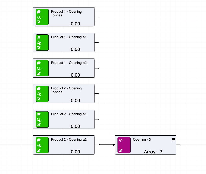
In this example, the calculation node contains multiple arrayrow() entries with each corresponding to a product and its quantities:
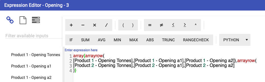
This can be repeated for both incoming and outgoing arrays. All three arrays can then be input into the storage node for calculations to occur.
The below calculations are specifically used to handle financial calculations.
| Function | Notes |
|---|---|
irr([values_node], start, end) |
Calculates the IRR for the given cashflow. Optionally provide the start/end to calculate the IRR for a range with in the model. Uses numpy-financial.irr internally |
irrall([values_node]) |
Calculates the IRR for all time periods, returning the same result at each period |
npv([rate_node], [values_node], start, end) |
Calculates the NPV of a given cashflow. Optionally provide the start/end to calculate the NPV for a range within the model. Uses numpy-financial.npv internally |
npvall([rate_node], [values_node]) |
Calculates the NPV for all time periods, returning the same result at each period |
pv([rate_node], [payment_node], start, end) |
Calculates the present value. Optionally provide the start/end to calculate the PV for a range within the model. Uses numpy-financial.pv internally |
pvall([rate_node], [payment_node]) |
Calculates the PV for all time periods, returning the same result at each period |
The rate node must be a single value such as a numeric node or fixed value. An error will be thrown if a timeseries or calculation node is used where the value differs between time periods.
NPV and PV behaves slightly differently to Excel. The calculation in the calc engine actually takes the NPV/PV from t = 1, then adds the value from t = 0 automatically. In Excel, this needs to be done manually
Listed below are additional calculations that have been added. Some overlap may exist with calculation engine v3 functions, but the entire set of calculations are documented here for completeness.
| Function | Notes |
|---|---|
isclose(first, second, [rtol], [atol]) |
This is based on the math function “isclose()”. Both the rtol and atol arguments are optional and default to 1e-09 for rtol and 0 for atol.Uses https://docs.python.org/3/library/math.html#math.isclose internally. |
| Function | Notes |
|---|---|
currentdayinmonth() |
The day of the month in the current period |
currentdayinweek() |
The current day of the week, where Monday == 1 and Sunday == 7 in the current period |
currentdayinyear() |
The current day of the year in the current reporting period |
currentmonth() |
The current month of the currently selected period |
currentperioddatetimeutc() |
The current period in UTC as an Excel based integer |
firstperioddatetimeutc() |
Similar to the above, but for the first period only |
lastperioddatetimeutc() |
Similar to the above, but for the last period only |
currentyear() |
The year of the currently selected reporting period |
datetimeexcelformat() |
Similar to currentperioddatetimeutc(), but named correctly for what it returns. This uses the openpyxl package to calculate the correct date |
daysinmonth() |
The days in the month of the current period |
daysinyear() |
The days in the year of the current period |
islastdayofmonth() |
Returns 1 if it’s the last day of the month for the current period, otherwise 0 |
islastdayofyear() |
Returns 1 if it’s the last day of the year for the current period, otherwise 0 |
currentfiscalquarter([start_month], [start_day], [start_year]) |
The current fiscal quarter. This defaults to Australian, but can be overridden by providing the start_month, start_day and start_year |
currentfiscalyear([start_month], [start_day], [start_year]) |
The current fiscal year. This defaults to Australian, but can be overridden by providing the start_month, start_day and start_year |
daysinfiscalyear([start_month], [start_day], [start_year]) |
The days in the current fiscal year. This defaults to Australian, but can be overridden by providing the start_month, start_day and start_year |
isfirstdayoffiscalyear([start_month], [start_day], [start_year]) |
Returns 1 if it’s the first day of the fiscal year, otherwise 0. This defaults to Australian, but can be overridden by providing the start_month, start_day and start_year |
islastdayoffiscalyear([start_month], [start_day], [start_year]) |
Returns 0 if it’s the first day of the fiscal year, otherwise 0. This defaults to Australian, but can be overridden by providing the start_month, start_day and start_year |
numperiods() |
The total number of periods. |
With the deprecation of Monte Carlo, it is important to highlight random functions and their abilities within calculation engine v4. There is no longer a distribution node. Instead, random nodes are created using standard calculations. They behave in a similar way to the old distribution nodes, however, they also have the option of returning an array of the distribution values, rather than just the single distribution value. In this case, a numeric seed must be passed in to the calculation either manually or through the use of a numeric node.
Seeds provide the ability to consistently return the same results for a particular random value. There are two ways of setting seeds. The first is creating a numeric value called SEED (note the case) which will be set at the global level and apply to all random numbers used by the model. The second is to pass the seed directly into the random calculation. Seeds do need to change per time period, otherwise each time period will have the same value. A calculation is applied to ensure that the seed is different per time period. Each time the model is run, the random number will be the same for each time period.
When a sample size is passed into the random calculation, rather than returning a single value, the calculation will return an array. The array will have one column, with an entry for each iteration returned by the underlying random number calculator. This is a very efficient way of returning a distribution of values, as it is not looping through multiple iterations like in calculation engine v3.
| Function | Notes |
|---|---|
normal(mean, sigma, [seed], [size]) |
Returns either a single value from a normal distribution, or an array of values |
continuousuniform(lower, upper, [seed], [size]) |
Returns either a single value from a continuous uniform distribution, or an array of values |
lognormal(mean, sigma, [seed], [size]) |
Returns either a single value from a lognormal distribution, or an array of values |
pert(minimum, mostlikely, maximum, [seed], [size]) |
Returns either a single value from a pert distribution, or an array of values |
triangular(lower, upper, mode, [seed], [size]) |
Returns either a single value from a triangular distribution, or an array of values |
weibull(a, [seed], [size]) |
Returns either a single value from a weibull distribution, or an array of values |
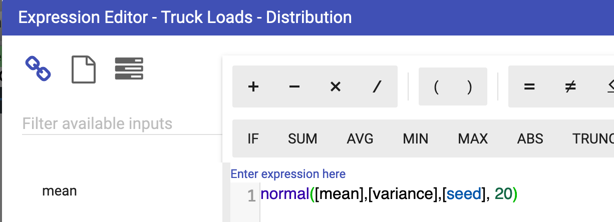
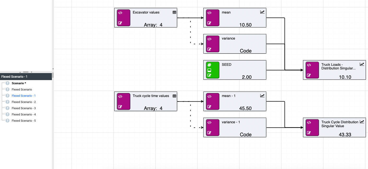
Using arrays with random calculations allows for the distribution of historical data to be approximated and passed into further calculations. A simple example being an approximation of the distribution of truck load sizes stemming from an excavator, and truck cycle times, to estimate the total tonnage moved within an operating day. See below for a basic example.
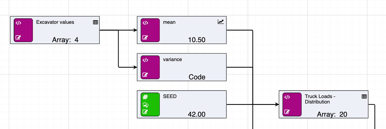
In this example, an array of excavator values takes the role of historical data from which the distribution is approximated. Ideally this would be a data source node with the customer’s real records. From this data, you can calculate the mean and the variance for input into the “Truck Loads - Distribution” node. In this example, the distribution is normal, but the parameters will be different depending on what distribution is being approximated. Noise can be added to both the mean and variance to increase the randomness and provide avenues for further testing.
The size parameter will determine the length of the array that is returned. This parameter can also be a node. Here you are returning an array of length 20.
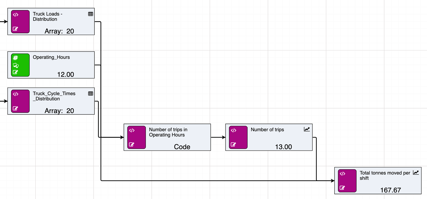
Similarly, this process can be repeated to approximate the truck cycle times.
Combined, the resulting arrays can be used to determine total tonnage moved within a specific time period by calculating the number of possible trips and summing the load values up to that point.
Similarly, random calculations can be used to generate single values from the distribution by omitting the [size] parameter.
If you wish to get a range of values, you can flex [seed] across scenarios for testing purposes.
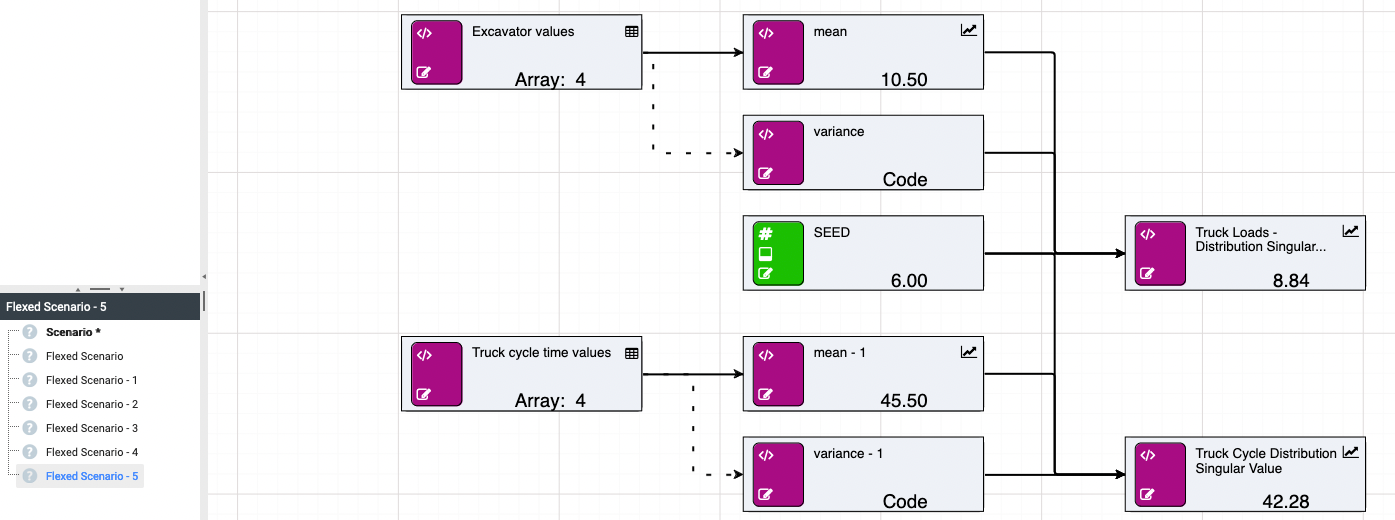
The SEED node will be automatically referenced by any random calculation within the scenario/model. This means the SEED node can be omitted from the function parameters.
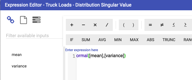
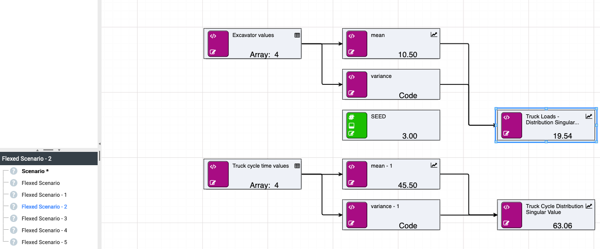
Random calculations will automatically detect the seed node, as long as the node name is SEED.
Subiterations provide a way of performing iterations for a group of nodes and then to return the output of those iterations.
They are structured similarly to components in that they have clearly defined boundaries using subiterationstart and subiterationend nodes.
The only difference with components is that it is not necessary to pass in nodegroups.
| Function | Notes |
|---|---|
subiterationstart(iterations) |
Defines the starting point of the sub iteration. The iterations variable is the number of iterations to run the group of nodes within the start and end boundaries |
subiterationinput([subiteration_start_node], "input_node") |
Gets the input node that has been fed into the subiterationstart() node for use within the subiteration loop. |
subiterationend([subiteration_start_node], [exit condition]) |
Defines the end point of the subiteration. The exit condition is optional and provides the ability to exit the subiteration early (e.g. if an iteration converges to a result). This can be used with the new isclose() function rather than == as an exit condition may be close enough to exit (i.e. the 40th decimal point might be different.) |
subiterationresult([subiteration_end_node], node_index_or_name) |
Gets the result feeding into the subiterationend() node. This can be by index (ordered by x and y coordinates) or by name. |
subiterationarrayresult([subiteration_end_node], node_index_or_name) |
This is the same as subiterationresult(), however rather than returning the last iterated value, this will return an array of the iterated values. |
subiterationcurrent() |
Returns the current iteration within an iteration loop |
The user interface in Akumen cannot display iterations as node values.
Therefore, it only displays the values as if there were no iterations (similar to components that display only the first nodegroup).
Stepping through time using the time slider DOES NOT step through the iterations, it steps through the time periods as if there were no iterations at all.
The iterations occur under the hood and are only exposed by the suberationeresult() calculation.
PriorValue nodes are used widely in Akumen to be able to fetch the value of a calculation from the previous time period.
The priovalue calculation has been improved to detect when it is within an iteration, and can be used to fetch the results of a calculation from a previous iteration.
Used in combination with isclose(), you can effectively check the last value compared to the current value to find convergence based on a boolean condition you define within the subiterationend() node.
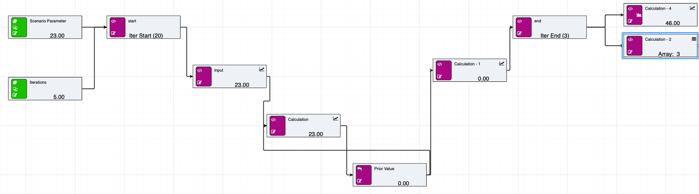
The above diagram is a simple example of a subiteration, with two inputs going into the subiteration. The start node shows that 20 iterations have been defined. The end node shows that there was an exit condition defined, and that it exited after 3 iterations. The two result nodes fetch the same calculated value, one returns the last value, the second returns an array of the 3 iteration values for the same result node.
The DatasourceArray formula allows users to extract rows in a Datasource filtered by date for each model period. This allows users to operate on categorical data, where multiple line items appear per date in a datasource, or to perform custom aggregation on data (for example, if the Datasource data is daily but the model is monthly).
The DatasourceArray formula returns an array with the relevant rows, returning an array with zero rows if no data appears in the selected period.
Note that only numeric columns will be returned, as arrays do not support non-numeric data.
| Function | Notes |
|---|---|
datasourcearray([Datasource Node], 'ColumnName') |
Basic Syntax of datasourcearray function. Will return an array with default row names (Row 0, Row 1, etc.). |
datasourcearray([Datasource Node], 'columns:ColumnName1, ColumnName2') |
Select multiple columns using a comma separated list. Will return an array with default row names (Row 0, Row 1, etc.). |
datasourcearray([Datasource Node], 'columns{;}:ColumnName1; ColumnName2') |
Specify a custom separator if there are commas in the column names. Will return an array with default row names (Row 0, Row 1, etc.). |
datasourcearray([Datasource Node], 'columns:all') |
Select all (numeric) columns. Will return an array with default row names (Row 0, Row 1, etc.). |
datasourcearray([Datasource Node], 'ColumnName', 'RowNameColumn') |
Specify a column to use for row names. Note that if the string in the third argument is not a column name, the string will be used as a prefix for the row names (e.g. datasourcearray([Datasource Node], 'ColumnName', 'CustomRowName')) which will result in the following row names:CustomRowName 0, CustomRowName 1, etc. |
datasourcearray([Datasource Node], 'ColumnName', 'RowNameColumn', 'FilterColumn1', 'FilterValue1', 'FilterColumn2', 'FilterValue2', etc.) |
Filter the returned rows in the same way as other Datasource calls. |
Range check calculations are a special type of calculation that allows the user to validate a node is within hard or soft limits. The node changes colour depending on it’s condition at each time period, and logs warnings in the error log if outside the limits.
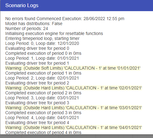
The log is accessible by right clicking a scenario and clicking on the view log button
In addition to colouring the nodes, there is another type of calculation called rangecheckresult([rangecheck_node]) that returns
-2 => below lowlow
-1 => below low
0 => ok
1 => above high
2 => above highhigh
Although Excel supports Circular References and there are times when it must be used, Circular References in Excel are not recommended due to the possibility of errors throughout the spreadsheet. Under the hood, Excel basically iterates through a number of times, and when it gets to the end of the iterations, that is your solution. Akumen’s Driver Models do not support circular references, except for Prior Value Nodes.
Prior Value Nodes are used to handle Circular References in Value Driver Models.
Prior Value Nodes can also be used to, in effect, create a recirculation, as shown in the example below.
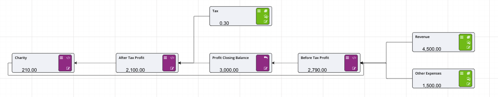
In this case we are not relying on iterations to give us the correct result, we are recirculating the charity back into the profit in the next time period.
At time t = 0, we have no profit, move the timeslider to t = 1 and we have the initial profit as in the example above using the optimiser. At time t = 2, the profit has circulated through and gives us our final after tax profit.
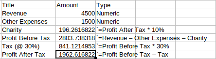
The calculations used in this are:
| Node | Description |
|---|---|
| Tax | A global node, used only as the tax rate for the profit calculations |
| Revenue | A fixed input node (though we could flex this through scenarios to do a what if on profit) |
| Other Expenses | Again, a fixed input node |
| Before Tax Profit | [Revenue] - [Other Expenses] - [Charity] |
| Profit Closing Balance | This is the prior value node - note there is no initialisation value for this for t = 0 |
| After Tax Profit | [Profit Closing Balance] * (1 - [Tax]) |
| Charity | [After Tax Profit] * 0.1 |
Note that in this example, Charity is calculated based on After Tax Profit, and it’s value is then used in Before Tax Profit.
Driver model nodes have the ability to execute other apps within Akumen, and retrieve the results. There are two basic use cases for this. The first is Driver Models can be componentised, that is, smaller well tested, purpose built driver models can be constructed that link together in a larger driver model.
Secondly, there are cases where driver models do not have the capabilities of a full language, such as Python. A Python application can be created, where the driver model can execute it, pass in values from the driver model, execute the Py (or R) model, and return the results back to the driver model.
There is a performance consideration for using Py/R apps within a driver model. Akumen still has to queue up the request to execute the Py/R app, meaning there is a short delay before the results are retrieved. A larger Py model can render the driver model almost unusable if the driver model must wait for the results to come back.
execute(app name, period, input1Name, [input1Node], ...)
where:
| Parameter | Description |
|---|---|
app name |
The name of the application to execute |
period |
set to 0 for Py/R models, as it is not used. For Driver Models, set to the period you wish to fetch |
input1Name |
The name of the input in the other app to execute |
input1Node |
The node who’s value will be sent to the application to execute under input1Name |
Multiple inputs can be specified, using the inputName, [inputNode] syntax
Executions cannot be chained together. For example, a driver model cannot call itself, and a driver model calling another driver model that also has executions will create an error.
The results from an execution can be fetched by creating a new node, and fetching the results using executeoutput.
executeoutput([executenode], outputName)
The executeNode is the node that is running the execute (as above), and outputName is the name of the output to fetch. An error will be thrown if the output does not exist. Multiple outputs can be fetched using multiple output nodes. Note that the execute caches the results, ie it will not re-execute every time an output is fetched, it will execute once, then the results will be cached for each output node.
This page describes the process for migrating a model from Calc Engine v3 (referred to as CEv3 from now on) to Calc Engine v4 (referred to as CEv4 from now on). For most cases this should be a relatively straightforward task, however there are some exceptions to this, for example where features in CEv3 are no longer supported in CEv4, or the syntax has changed.
CEv3 is still available and can be kept as the engine running your CEv3 models, so migrating is optional.
All existing driver models will continue to use CEv3. Any new driver models will use CEv4.
It is recommended to do the migration in a clone of your existing model so you have a copy on hand to revert back to if required.
To change the calc engine version, open the Application Properties window.
This can be done by right-clicking the model on the Application Manager and selecting Properties or by selecting the model properties gear from within the model as shown below.
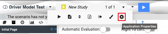
In the Properties window, select the Configuration tab:
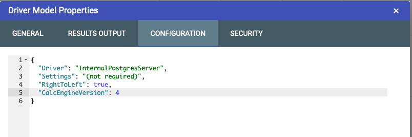
Add the following line to the configuration as per the example above, also ensuring that a comma has been added to the end of the previous line:
To revert back to CEv3, change the 4 in the line above to a 3 or alternatively remove the “CalcEngineVersion” line.
Some node types have been removed in CEv4.
When an unsupported node from CEv3 is used, and converted to CEv4 the UI will display an error indicating the node type is no longer supported:
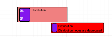
Distribution nodes are not supported by CEv4 and have been removed. An alternative is to use the new random calculations from section Functions & Operators.
Spreadsheet Nodes/Spreadsheet Input Nodes/Spreadsheet Output Nodes are not supported by CEv4. If your CEv3 model contains Spreadsheet Nodes, you will need to replace these with other node types. If your spreadsheet nodes contain only numbers (i.e. have no formulas), consider using Asset Nodes, Numeric Nodes, Timeseries Nodes or Datasource Nodes as a replacement. If your spreadsheet nodes contain model logic (i.e. have formulas), you will need to extract that logic into calculation nodes.
CEv4 implements a few changes in syntax to enforce a stricter standard when writing calculations. If your calculations work in CEv3 but error in CEv4, check this section for known changes in syntax in CEv4.
CEv3 treats any text in between commas in a function call as a string and supports the following call:
In CEv4 this throws an invalid syntax error, and would require the user to put quotes around the parameter to succeed as per below:
This will happen for all non number/letter characters present in these parameters. This will mostly affect datasource calls as the filtering function is free text.
CEv3 accepts node names in calculations with leading and trailing spaces.
For example, the nodes “My Value” and “My other value” could be called in a calculation as:
In CEv4 the matching is stricter and will not accept this:
In CEv3, it is possible to reference single-word node names in calculations with and without using square brackets. For example, a node called “MyValue” can be referred to as follows:
This is not supported in CEv4. Square brackets are required when referencing nodes in calculations as follows:
Some of the new functions for CEv4 are dynamic, in that they dynamically build their inputs based on the connected inputs
rather than having to fix the inputs in the calculation string. This is useful for building components, or knowing there may be new nodes in the future.
Functions that support dynamic inputs will be labelled as such in the documentation. To use them, simply leave the calculation with no parameters (e.g. array()).
The order nodes are laid out on the page matters for dynamic functions, such as node groups and arrays. When referencing nodes by index, the order the nodes are listed is determined from their positions on the driver model canvas - first by the y-axis, then by the x-axis.
Some of the special calculations (e.g. those that hold multiple values, such as arrays, component inputs or python nodes) don’t display the individual values like in calculation engine v3. These cannot be used directly in calculations and must be called upon by their helper nodes.
The calculations in this section are deprecated and only available when using Calculation Engine v3.
This functionality is only supported in Calculation Engine v3.
| Function | Notes |
|---|---|
optimise(numParticles, maxIterations, [evaluationnode], targetvalue, [first_input], first_input_lower_bound, first_input_upper_bound, ... to max of 5 inputs) |
Optimises a node, altering inputs until the target value is reached |
optimiseerror([optimise node]) |
Returns the error, ie how far from the target value was reached |
optimiseInput([optimise node], [Input node]) |
Returns the final input value from the optimisation |
minimise(numParticles, maxIterations, [evaluationnode], [first_input], first_input_lower_bound, first_input_upper_bound, ... to max of 5 inputs) |
Alters inputs until the minimal value of the result node is reached |
minimiseInput([minimise node], [Input node]) |
Returns the final input value from the minimisation |
maximise(numParticles, maxIterations, [evaluationnode], [first_input], first_input_lower_bound, first_input_upper_bound, ... to max of 5 inputs) |
Alters inputs until the minimal value of the result node is reached |
maximiseInput([maximise node], [Input node]) |
Returns the final input value from the maximisation |
This functionality is only supported in Calculation Engine v3.
The Optimiser functionality can be used as an option to handle Circular References in Value Driver Models.
You can use the Optimiser to in effect perform circular calculations if there is no mathematical way of solving the problem using standard nodes (within the current time period). Take the example below.
There is a circular reference in that the donation to charity is based on the after tax profit, but the profit also includes the donation to charity as a component of revenue - other expenses - charity.
The design pattern in Driver Models looks as follows:
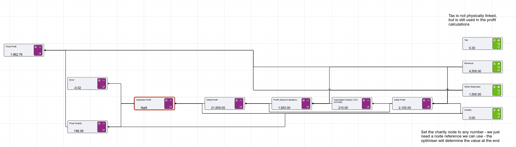
Lets step through this node by node:
| Node | Description |
|---|---|
| Tax | A global node, used only as the tax rate for the profit calculations |
| Revenue | A fixed input node (though we could flex this through scenarios to do a what if on profit) |
| Other Expenses | Again, a fixed input node |
| Charity | This is an interesting node, in that we do not set a value. It is, however, required to exist to be used by the optimiser. |
| Initial Profit | ([Revenue]-[Other Expenses]-[Charity]) * (1 - [Tax]) |
| Calculated Charity | [Initial Profit] * 0.1 |
| Profit (Second Iteration) | ([Revenue] - [Other Expenses] - [Calculated Charity (10% of Profit)]) * (1 - [Tax]) |
| Delta Profit | ([Initial Profit] - [Profit (Second Iteration)])^2 |
| Optimise Profit | optimise(15, 20,[Delta Profit], 0, 9, [Charity], 0, 2000) |
| Error | optimiseerror([Optimise Profit]) |
| Final Charity | optimiseinput([Optimise Profit], [Charity]) |
| Final Profit | ([Revenue]-[Other Expenses]-[Final Charity]) * (1 - [Tax]) |
The idea is that we calculate an initial profit. Note that the entered charity can be any value - this value will not get used, but the node reference will be used by the optimiser. We then calculate charity, and the second iteration for profit based on this charity. Once we have the second iteration, we can calculate a delta. Note that we raise to the power of 2 to avoid issues with negative numbers.
This is where the optimiser comes in - we want the delta between the initial profit and the second iteration of profit to be 0, by modifying the charity. We can take a guess at the range the charity should be to set the lower and upper bounds. If we hit 0, we’ve got an optimal solution. We can double check that using the error node - this should also be 0. We can then use the optimiseinput calc to retrieve the input charity value, and finally calculate a final profit.
Notice that the Optimise node is highlighted red. Hovering over the node shows that the number of iterations defined (20) is not enough to solve to 9 decimal places. Given this is currency, we can change the optimise node calc to solve to 2 decimal places. Turning Automatic Evaluation on and off will continue to solve - you’ll notice at this point that the final profit changes slightly when this occurs. This is because there could be multiple solutions to the problem, resulting in slightly different results.
This functionality is only supported in Calculation Engine v3.
Akumen has a calculation function for performing basic optimisations. Optimisations come in 3 types:
The syntax for Optimise is:
optimise(numParticles, maxIterations, [evaluationNode], targetValue, solvePrecision, [first_input], first_input_lower_bound, first_input_upper_bound, ...)
The syntax for Minimise and Maximise is:
minimise(numParticles, maxIterations, [evaluationNode], [first_input], first_input_lower_bound, first_input_upper_bound, ...)
maximise(numParticles, maxIterations, [evaluationNode], [first_input], first_input_lower_bound, first_input_upper_bound, ...)
where:
| Parameter | Description |
|---|---|
numParticles |
This is the size of the solution space. Start of small (eg 10), then work up from there. Remember, the larger the solution space, the longer it’ll take to solve |
maxIterations |
The maximum number of iterations before the solver will stop. Again, start of small, and if it’s not solver increase this. Note that this will also impact on performance of your driver model if it’s too large |
evaluationNode |
This is the node that will be evaluated, ie the objective function |
targetValue |
Only used for the optimise mode - the value that the optimiser will try and hit |
solvePrecision |
Only used for the optimise mode - precision to use when trying to hit the target, for example 2 would solve to 2 decimal places |
first_input |
The first input to use in the solve |
first_input_lower_bound |
The lower bound (constraint) of the first input |
first_input_upper_bound |
The upper bound (constraint) of the first input |
The minimum requirement is one input. If any more are required, follow the same pattern as above - input, lower, upper.
There is a hard maximum of 5 inputs that can be used to perform an optimisation
There are performance implications on large settings for numParticles and maxIterations. Ensure these are set at an appropriate level to manage the performance of the driver model.
Occasionally the min/max or optimised value is not the only result that is required. You might also need to access the inputs that were used to generate the optimal result. This can be done using a second calculation node, and using:
optimiseinput([optimiseNode], [optimiseInputNode])
minimiseinput([minimiseNode], [minimiseInputNode])
maximiseinput([maximiseNode], [maximiseInputNode])
To determine if optimise has converged, create a new calculation node using the following expression:
optimiseerror([optimiseNode])
This will show how far away from the target value was achieved.
Prior value nodes are a special type of node used mainly in timeseries type driver models that model a starting balance and ending balance. Examples include things such as stockpiles, tank levels etc. Calculations can be used to “recirculate” back into the opening balance at the next timestep. This is a way of avoiding Circular References
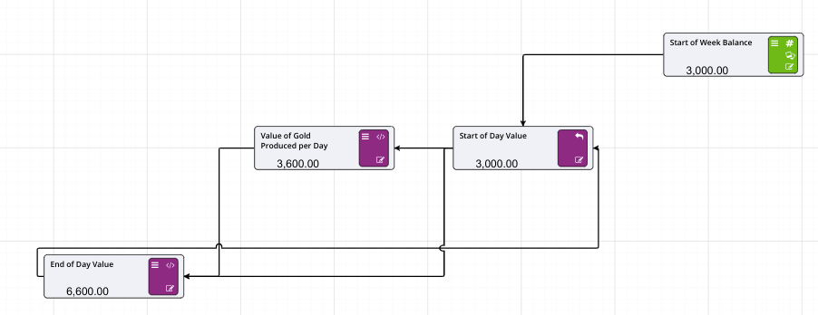
A prior value node can be added using the  icon. It is configured using input and output links, rather than any configuration settings per se.
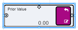
The Prior Value node has two input ports, and one output port (hover over the ports for a description on the function they perform). The first input port is at the top of the node and is the initialisation value, that is, the opening balance prior to time 0. Normally a scenario input would feed into this port. It can be left without an initialisation value, in that case the value will be 0.
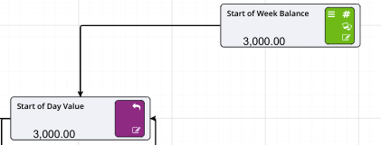
The output of the prior value node feeds into another calculation to calculate the daily amount. It in turn feeds into a second calculation which is the end of day value, that is, [Start of Day Value]+[Value of Gold Produced per Day].
Lastly, this end of day value loops back into the Start of Day Value prior value node.
Akumen pages is a useful tool for separating logic of a driver model. Without a way of showing how a particular calculation gets it’s value, it is difficult to follow the driver model logic, especially on larger driver models.
The node reference provides this functionality.
By using a Node Reference instead of a Numeric node or using a repeat node means that if a change is made to the node being referenced the change is pulled through to the Node Reference.
So for example if you had a Driver Model that worked out the monthly income for a coffee shop on one page, and the monthly expenses for the same coffee shop on another page, you could use both results on in the main Driver Model by using Node References. The results of both calculations would be passed through to the main Driver Model through the Node References allowing them to be used in a calculation which works out the cash flow for the month (see Figure below)
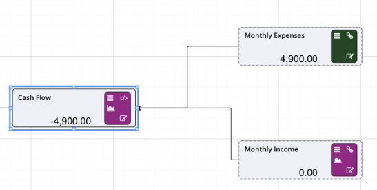
To set up a Node Reference:
 onto the workspace.
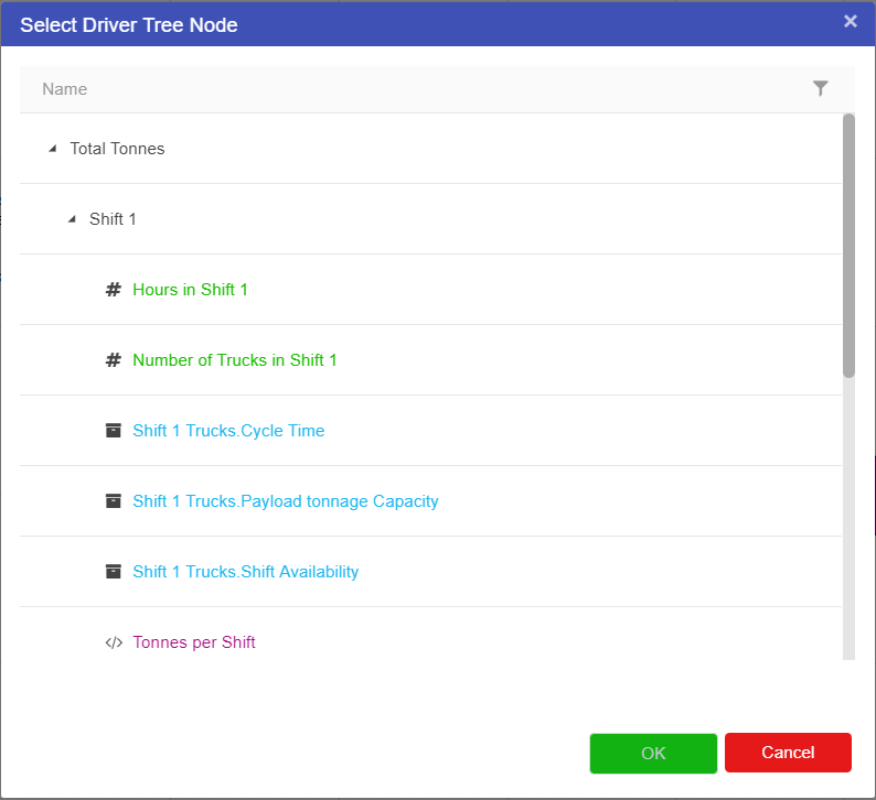
To reconfigure a Node Reference, access the properties of the reference node. The property pane looks as follows:
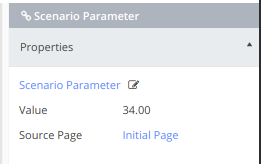
Clicking on the name of the linked node will navigate to the page the node resides on, and highlights the node. Clicking on the Source Page navigates to the source page without selecting the node. Clicking the edit button pops up the node selecion dialog and allows you to point the reference node to a different node.
Note that this does not update any linked calculations, it only physically changes the links. Any calculations pointing to the reference node need updating.
A Label node is a essentially a free text box node. It allows users to place text on the workspace to describe nodes, and leave notes on the workspace.
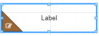
To edit the text of a label node just click on the text and start typing.
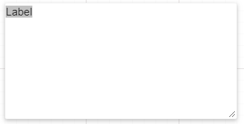
If users want to change any of the properties of the text within the node click on the edit symbol at the bottom left of the node, and the properties for the node will appear on the right of the screen.

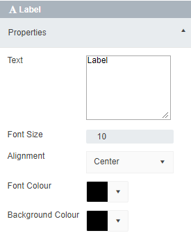
Label nodes do not automatically change size when text is entered. Users will have to resize the node to fit the text entered.
In addition to entering plain text into the label, the labels also support calculation nodes. The same expression format as in the calculation Expression Editor eg My node: [NodeName] will replace the [NodeName] with the results of the calculation.
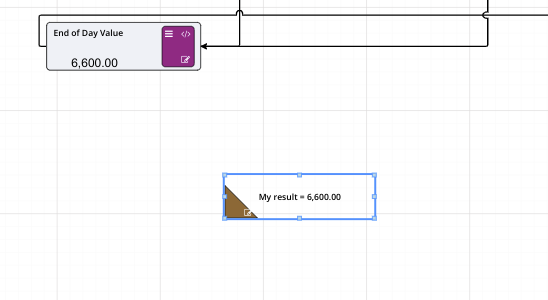
Image nodes serve the same purpose as Label Nodes in that they exist to help users navigate a Driver Model.
To add an image node, click on the image node icon  . Once the image node is on the workspace, the default image will load onto the screen and a Select Image screen will appear allowing users to change the image in the node.
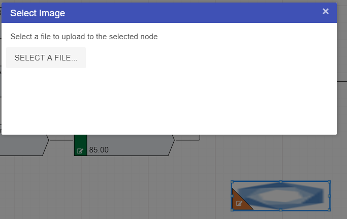
Once the image is uploaded to the node, the node will display the image. Like the Label node it can be resized and adjusted as much as the user likes to fit the Driver Model.
Background image nodes serve the same purpose as Image Nodes in that they give context to the Driver models.
To add a background image node, click on the background image node icon ![]() . Once the background image node is on the workspace, the default image will load onto the screen and a Select Image screen will appear allowing users to change the image in the node.
. Once the background image node is on the workspace, the default image will load onto the screen and a Select Image screen will appear allowing users to change the image in the node.
An image file can be uploaded from your device to the background image node. After the image has been uploaded, its position can be locked and unlocked. If the node is locked, it will prevent you from moving or resizing the image.
Datasource nodes allows data from datasources to be efficiently brought into the Value Driver Model. There is a prerequisite, and that is the data must be time based, that is, one or more columns must be of type timestamp.
The datasource node itself can be thought of a linking node and a pre-filter. Dragging a datasource node (via the lightening bolt node icon in the palette) pops up the following window.
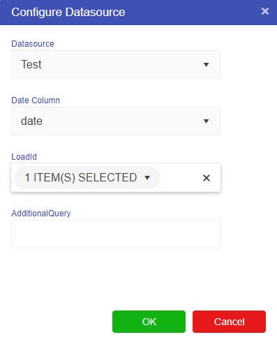
The two required fields are the Datasource and the date column. The date column must be of type timestamp within the underlying table, otherwise the datasource cannot be created.
The two optional fields are the Load Id and the additional query. More than one load id can be specified, with the data filtered by that load id.
Once the datasource node is created, clicking on the lightening bolt on the node itself will open the datasource viewer (the same viewer as the main datasource configuration).
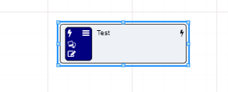
If the load id and/or query is configured, the viewer will automatically be setup to use those settings. Also in the viewer, clicking on the upload button will redirect back to the Datasources configuration page and the upload window will popup, preconfigured with the first selected load id.
Once the datasource node has been configured, it can be used in the special datasource(...) calculation nodes (see here for full syntax).
Datasources can be loaded in any time period. For example, you may have daily data, but your Value Driver Model might be monthly. Or you may have hourly data and the VDM has daily data. Akumen handles this by allowing the data you ingest to remain in it’s raw form, then automatically aligning the data to the time periods in the Value Driver Model. The only caveat with this is the start and end time of the driver model need roughly align with the time periods in the datasource data.
The datasource calculations allow you to define the aggregation method to roll the data up to same time periods as the Value Driver Model.
The forward fill options allow you to either error the model, or forward fill the data replacing missing data with the last known value or an arbitrary value.
Finally the filters allow you to target specific rows within the datasource. For example your datasource may have OSI PI data, with multiple tag/timestamp/value compbinations of data. The you may want a particular calculation to fetch tank 1 data, but not the data from the rest of the tags.
Akumen is smart enough to decide what exactly is required for the list of VDM calculations, and only fetch the minimum data required to meet the needs of the Value Driver Model.
The following nodes are deprecated and only supported in Calculation Engine v3:
The Distribution node in Akumen is actually a user defined Monte Carlo simulation node. Drag a distribution node from the palette, select the node properties and enter a mean and standard deviation, and then execute the model to get a standardized value as a result.
A Monte Carlo simulation is a simulation that performs risk analysis by substituting a range of values based off a probability distribution for any factor that has inherent uncertainty. It calculates an average result based off a different set of random values.
The number of random values used is controlled by the number of iterations set. An iteration is the number of times a calculation is performed to find the best possible average value. The default number of iterations for each model is 100, the hard limit for the number of iterations * the number of time periods is 10000.
The more iterations users have in the model the more accurate the average result will be. However, it will also take the model longer to run.
There is a hard limit of how many iterations and time periods are available, which is 10000. This is calculated using the number of iterations * the number of time periods. The model will not allow a value outside this range to be saved, so consider adjusting either the iterations or time periods. For example, if a user used the default iterations of 100, and specified 99 time periods, that would be 9900 iterations, and is allowed. Specifying 1000 iterations would exceed the available iterations.
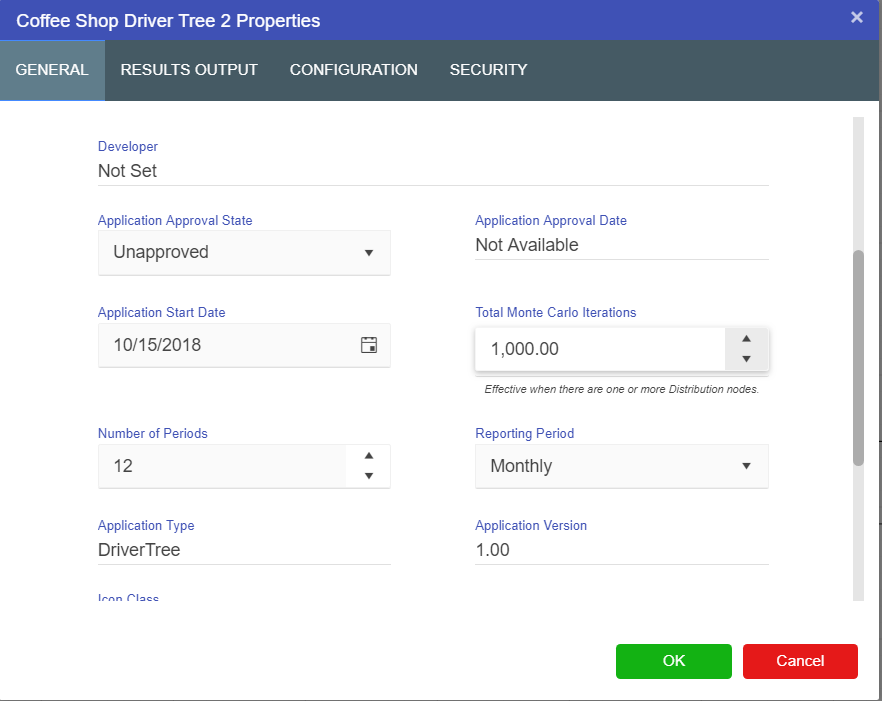
The Distribution node in Akumen supports five distribution types:
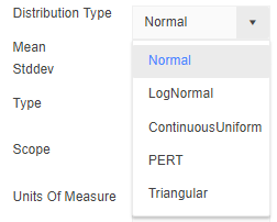
Each Distribution node will require users to:
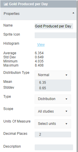
When a scenario is not executed, the distribution’s user entered mean value is used in automatic evaluation. Once the scenario is run and results generated, additional calculated values will appear in the distribution properties. Also any calculation using the distribution will now use the calculated mean value.
The Distribution node will allow you to change your distribution type but will not automatically refresh the requirements. To get the correct requirements:
You will then be able to enter the required values to find the average value of any distribution.
To set up a Distribution node:
 onto the workspace.
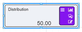
 on the bottom left of the node.
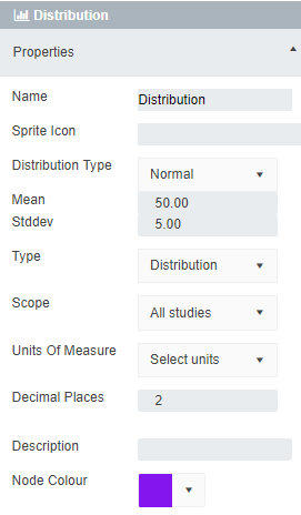
Once both have been entered the node will calculate the initial value of the distribution. To get the average value of your Distribution node you must execute the scenario.
Spreadsheet nodes are deprecated functionality and will be removed in a later release of Akumen. This node type can only be used with the v3 calculation engine and is not supported in calculation engine v4.
Spreadsheet nodes allow for spreadsheet functionality inside a Driver Model.
There are three types of Spreadsheet nodes:
Spreadsheet Inputs - directs the incoming value to a specific cell within the spreadsheet node;
The Spreadsheet - the actual spreadsheet data; and
Spreadsheet Outputs - directs a specific cell’s value to be outputted from the spreadsheet so it can be used in calculations.
The Spreadsheet node acts just like an Excel spreadsheet. Within it you can:
The spreadsheet node only allows inputs from the Spreadsheet Input node and only outputs to the Spreadsheet Output node. The spreadsheet input and output nodes define the sheet, cells and configuration required to feed data into the spreadsheet, and pull data out of the spreadsheet. The input node accepts a single input, feeding the data into the spreadsheet, while the output node has a single output, pushing the data into the next calculation in the VDM.
Dragging a spreadsheet node from the palette using the  symbol will automatically open the spreadsheet interface.
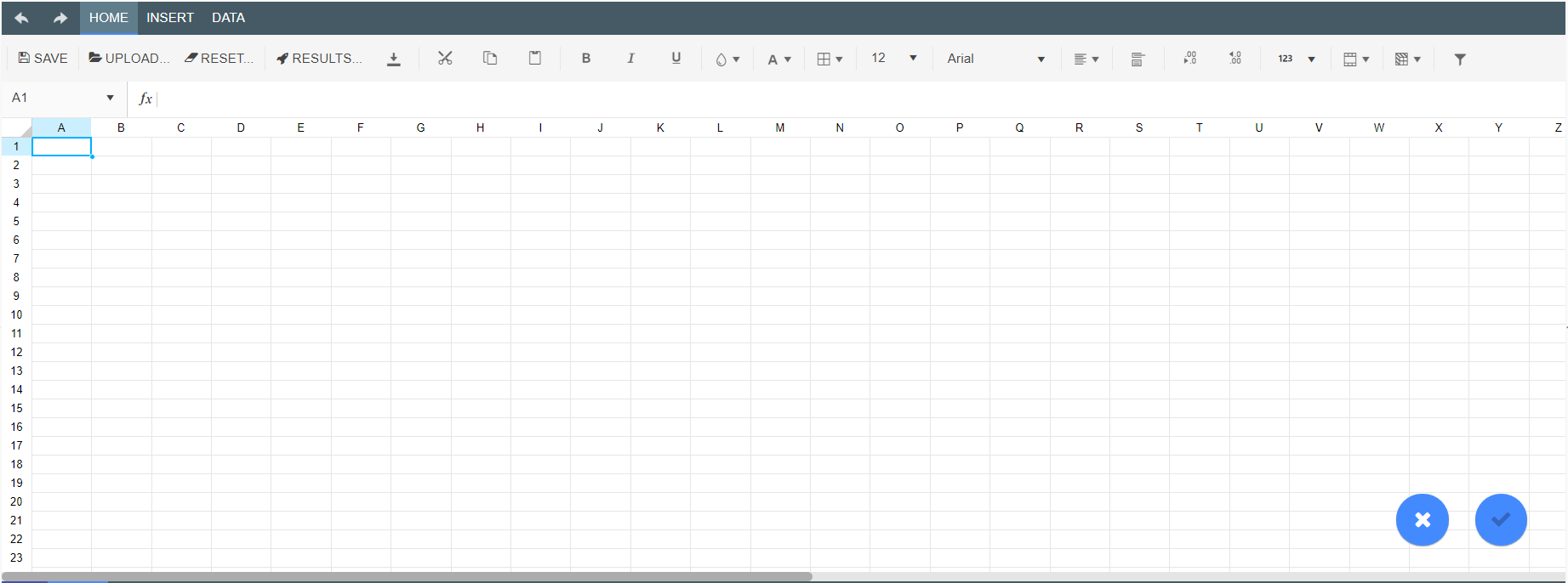
To exit out of the Spreadsheet node select the Exit button at the bottom right of the screen next ot the Save button.
Once a Spreadsheet Input node has been connected to a Spreadsheet node users will be able to go into the Spreadsheet node and manipulate the data that has been input into the spreadsheet.
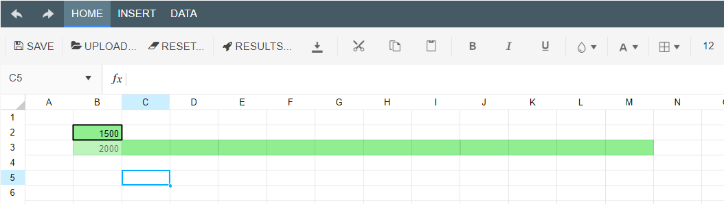
A Spreadsheet node can be simple or complex, it behaves as an excel spreadsheet and can have its data manipulated in the same way it can be manipulated in excel. Once the data has been input into the spreadsheet users can label the input data simply by typing as if it were a normal spreadsheet.
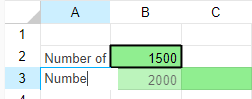
Users can also resize columns and rows, enter in new values, and even enter in equations.
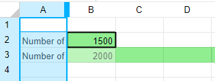
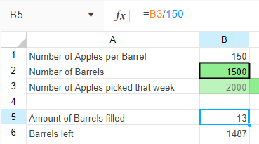
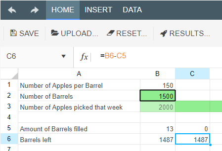
Using the Results button, the spreadsheet node can be used to replace the contents of the current spreadsheet with the results of another driver model, or even a Python or R model. Note that the other model must be fully executed and results generated.
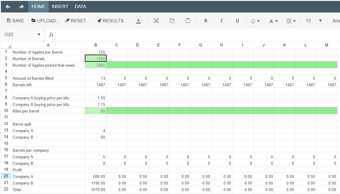
Spreadsheet nodes are deprecated functionality and will be removed in a later release of Akumen. This node type can only be used with the v3 calculation engine and is not supported in calculation engine v4.
The SpreadSheet Input node takes values from other nodes in the Driver Model and pushes them into a spreadsheet. It can take any value from any node and transport it into the spreadsheet.
There are two types of ways to put values into the sheet:
A Spreadsheet Input node will not take any input values until it is connected to a Spreadsheet node. Only once connected will users be able to set where input values go in the spreadsheet.
A Fixed value means that the value does not change over time. The value is set into a cell in the spreadsheet and that it does not populate the other cell values.
A Timestep value is one where a new value can be obtained over a number of time periods. They work best when a Timeseries node is attached to the Driver Model.
The purpose of the Spreadsheet Input node though is to take inputs and push them through to a spreadsheet. You cannot edit the spreadsheet in this node, only supply where inputs need t go into the spreadsheet.
To step up a Spreadsheet Input node:
 symbol onto the workspace.
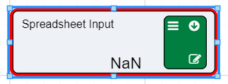
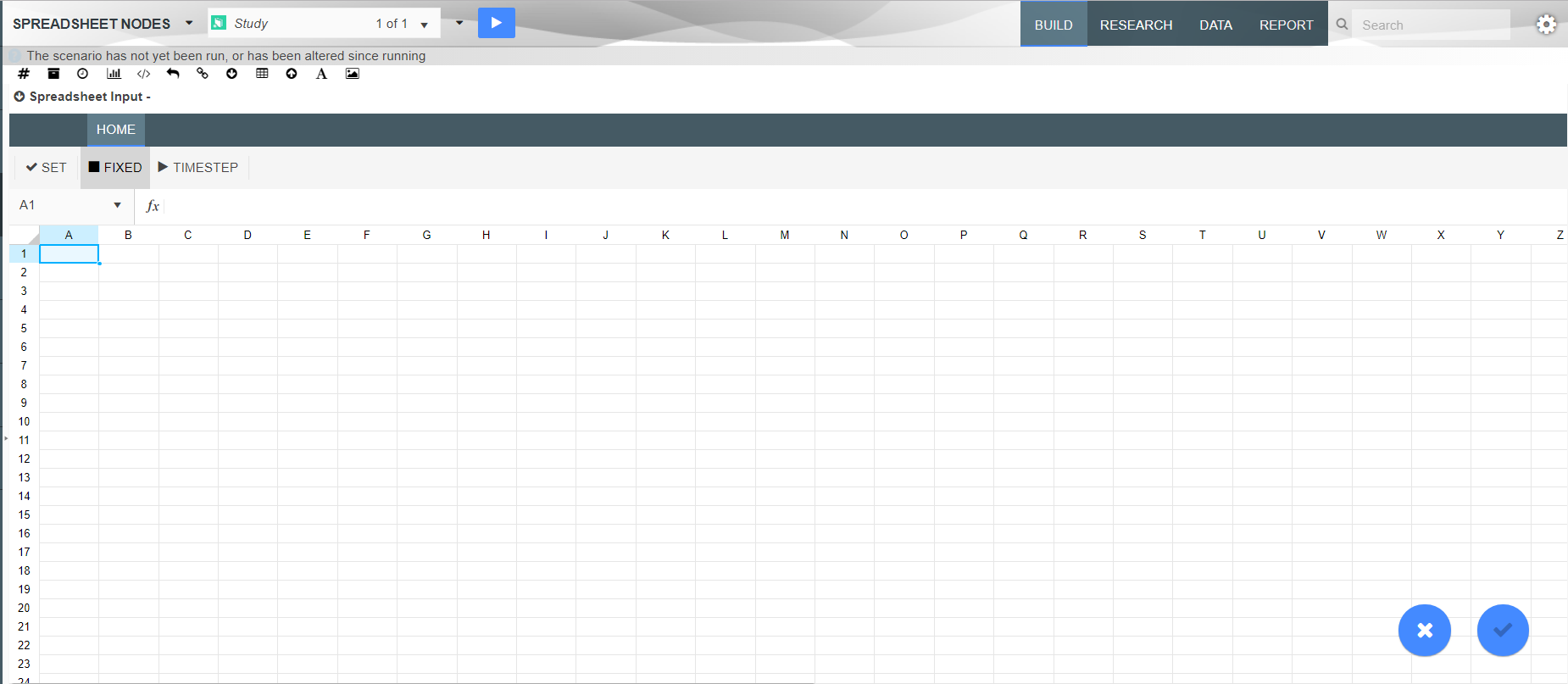
If the input is a fixed value:
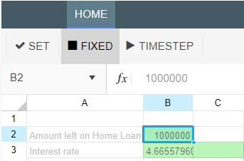
If the value is a timestep value:
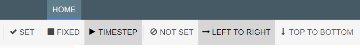
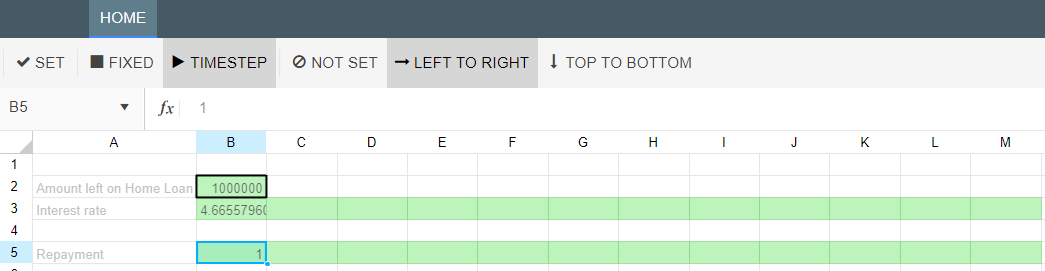
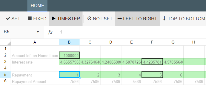
Spreadsheet nodes are deprecated functionality and will be removed in a later release of Akumen. This node type can only be used with the v3 calculation engine and is not supported in calculation engine v4.
Once a spreadsheet has been created inside the Spreadsheet node, users will need to retrieve the Outputs in order to use them in the Driver Model. As mentioned on the Spreadsheet node page, a Spreadsheet node will only output to a Spreadsheet Output node.
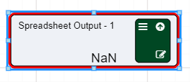
A Spreadsheet Output Node is exactly the same as a Spreadsheet input node, except instead of giving inputs it take results from the spreadsheet for use.
Like a Spreadsheet input node the outputs delivered can be a timestep value or they can be a fixed value.
To set a value to be output from the spreadsheet for use:
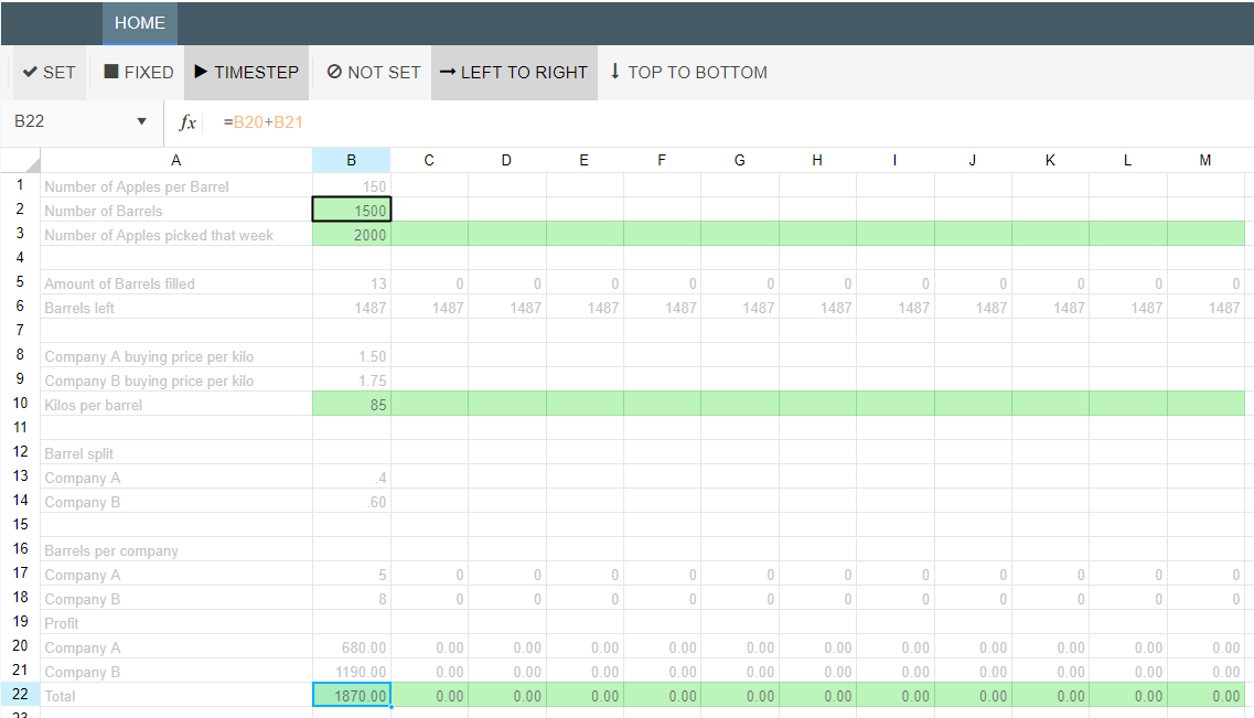
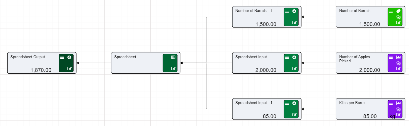
Nodes can be changed between types. One of the most common use cases is to change an asset node type to a numeric node type.
To change a node from one type to another, access the node’s property grid, and change the type, as shown below.
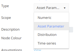
In this example, we’ll demonstrate how to convert an asset to a numeric.
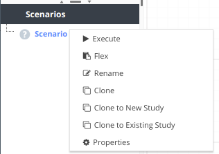
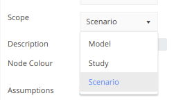
Note that when flexing on asset parameters, the flexing process will automatically convert flexed scenarios from Asset to Numeric as well as set the scope to Scenario level. Flexing parameters can be performed from both the Driver Model interface, as well as the Research grid.
To create a new Code Model:
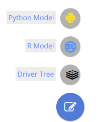
There are few extra things to note about the creation of Applications in Akumen. The first is that if you leave your application at any time you can always get back to it by either going through the APPS section again or the RECENTS tab. Both will take you straight back to your Model.
If you are looking at the Application Manager screen you will also notice how there is an icon that has three vertical dots at the right end of each App.
If you click on the above icon the following options will be brought up:
Multiple files and folders can be created in the file explorer to the left. To specify the main entry point for Akumen, one of the files must be specified as the execution file. The first file created is set by default as execution file. It can be changed to an other suitable file from the context menu in the file explorer. The execution file must contain the Akumen function called “akumen”.
Python and R applications in R utilise code comments in the execution file to define the inputs and outputs required for the model. Note a sample is automatically created when a new model is created.
Python applications in Akumen are run “headless”, i.e. without a GUI. That means, if libraries like matplotlib are used in the app code, a non-interactive backend has to be chosen. For example:
When the first file is created in the new app, the akumen function is created. The top section contains code comments, which are used to construct the inputs and outputs required to “wire” the parameters into Akumen. These follow a specific format, as shown below.
Python applications require a function in the form def akumen(first, second, **kwargs).
For example:
Or:
R applications require a function in the form akumen <- function(first, second, ...) {}.
For example:
All parameters are defined in code comments at the beginning of the akumen function in the execution file.
Input parameters are defined must be defined in one of the following ways:
Input: name [float]Input: name [int]Input: name [string]Input: name [datetime]Input: name [json]Input: name [tabular]Input: name [file] (csv)Input: name [enum] (enumTypeName)Input: name [list]Input: name [assetview] (optionaltype)Input: name [assettemplate]Input: name [scenario]Input: name [datasource]Parameter names must be unique (whether input or output) per application. Inputs are copied to outputs and are available in reporting and analytics.
Setting the correct datatype will change the editor in the research tab to the appropriate editor for that datatype.
| Type | Description |
|---|---|
[float] |
Specify the scenario value inline in the research grid (Optional: use [float:2] to specify 2 decimal places |
[int] |
Specify the scenario value inline in the research grid |
[string] |
Specify the scenario value inline in the research grid |
[datetime] |
A date-picker appears when the cell is selected in the research grid |
[json] |
Define a json structured input via the cells right click menu |
[file] |
Access the Akumen document select/upload dialog via the cell"s right-click menu |
[tabular] |
Define tabular data in a spreadsheet interface via the cell"s right-click menu. This can be used to define timeseries inputs or any other table of regularly-structured tuplets |
[enum] |
Enum inputs require the enum to be created in Akumen, with enumTypeName referring to the name of the enum. |
[list] |
Define list data in a spreadsheet type interface via the cell"s right-click menu |
[assetview] |
Defines the name of the asset view to use within a model, and links the application to the view so that the view cannot be deleted. |
[assettemplate] |
Defines the name of the asset template to use within an application |
[scenario] |
Pops up a picker for selecting an Application, Study and Scenario name, and adds them to the application as a JSON structure |
[datasource] |
Pops up a picker to allow a connection to a datasource, selection of one or more load ids and an optional additional query |
Note that there is a maximum size limit on tabular inputs of 2mb. If you want to use a dataset larger than this, supply it as a file input instead! Tabular is primarily intended for inputs that are manually created/modified through Akumen, or small sheets that may need some manual data entry before use.
Output parameters must be labelled like one of the following, and will be outputted to the AppOutput table (unless there is a ParameterGroup defined):
Output: name [float]Output: name [file] (file_name.csv) {fieldname:datatype[,fieldname2:datatype2...]}Output: name [file] (file_name.csv) {Column1:string,Column2:float,Column3:int}Note that (file_name.csv) is now optional.
Output: name [tabular] {fieldname:datatype[,fieldname2:datatype2...]}is equivalent to
Output: name [file] {fieldname:datatype[,fieldname2:datatype2...]}To mark a generated file for import into Akumen the output parameter would be declared as:
Output: fileparam [file] (hourly_data.csv) {fieldname1:float, fieldname2:boolean}This will load the values from the file hourly_data.csv into the table hourly_data.
If no column output types are specified in the output types above, the type will be inferred from a small subset of rows in the data.
Tabular and Scenario outputs can both select scenarios from other applications. This list by default pulls all apps and studies, however it can be controlled by adding in the following configuration items:
{allowed_app_list=comma separated list of app names}{allowed_study_list=comma separated list study names}Note that the app list filter can be used without the study list, but the study list cannot be used without the app list .
Controlling whether or not parameters appearing in the research grid can be setup using the following syntax:
{publishtoresearch=true} or {publishtoresearch=false}
For example, an output parameter may be included using:
- Output: name [float] {publishtoresearch=true}
The default for Python/R models is that all parameters appear on the research grid.
Controlling whether Akumen based outputs appear in the AppOutput structures can be set up using the following syntax:
{publishtoappoutput=true} or {publishtoappoutput=false}
For example, an input parameter may not be required in the AppOutput,
- Input: name [float] {publishtoappoutput=false}
Controlling the grouping of parameters into different AppOutput “tables” can be setup using the following syntax:
{parametergroup=groupname}
All parameters with the same group will be loaded into a table called AppOutput_ParameterGroup. Use this when there are too many parameters to be realistically used on the research grid (> 1000).
The research grid will display a maximum of 50 columns, even if more are marked as visible.
Controlling whether results are persisted, rather than deleted, are controlled using the following syntax:
{persist=true} or {persist=false}
This provides the ability to retain results between runs, rather than clearing results.
When using the persist flag and if there is a chance of duplicates when running the app as a scheduled app, the duplicate column key can be defined using the following syntax:
{duplicatekey=col1,col2}
In other words, a comma separated list of column names in the expected data set.
The friendly name of the parameter (displayed in any templated pages) is configured using the following syntax:
{description=friendlyname}
Finally, the outputs must be returned from the R/Python specific return function.
Additional variables are available for each model run. In Python, these are accessible through the akumen_api module, e.g.
In R, these are included when you add source('akumen_api.r') to your code:
| Variable | Description |
|---|---|
AKUMEN_URL |
The base Akumen url |
AKUMEN_API_URL |
The base url of the Akumen API - this is the most commonly used URL for API access |
API_KEY |
The api token for API access - this is set based on the context of the current user of Akumen OR the runas user for a scheduled app |
MODEL_NAME |
The name of the currently executed application |
STUDY_NAME |
The name of the currently executing study |
CLIENT_NAME |
The name of the client the currently executing user belongs to |
STUDY_ID |
The unique identifier of the study, useful when creating customized databases in Akumen and linking to a study |
SCENARIO_NAME |
The name of the current executing scenario |
SCENARIO_ID |
The unique identifier of the scenario, useful when creating customized databases in Akumen and linking to a study |
SCENARIO_CONFIGURATION |
JSON dictionary of scenario configuration - can be anything required by an application, and set through scenario properties |
IS_BASELINE |
True or False flag indicating if this is the baseline scenario for the study |
MODEL_START_DATE |
The configured start date of the model |
MODEL_END_DATE |
The configured end date of the model |
SCENARIO_START_DATE |
The configured start date of the scenario |
SCENARIO_END_DATE |
The configured end date of the scenario |
| - | |
| Python only: | |
progress(message) |
Function to provide a progress indicator. Each message provides the time in the logs it took to execute the message, and is constantly updated (and returned) back to Akumen |
Python models are also able to access a number of helper functions that are designed to ease the use of the Akumen API and other endpoints in modelling. These functions are described below.
get_results_views(model_name)Retrieve a list of all data views associated with a model, for use with get_results().
model_name: string: name of the modellist: list of view namesget_model(model_name)Returns metadata about the model, including study and scenario details.
model_name: string: name of the modeldict: model detailsget_results(source, view_name, scope='scenario', query='')Get the results of a source model/study/scenario and return as a dataframe.
source: Akumen Scenario input {"model_name":"...","study_name":"...","scenario_name":"..."}view_name: Name of the results viewscope: Scope of results to retrieve [model, study, scenario]query: Filter query stringDataFrame: Pandas DataFrame containing resultsThe following helpers are not included in the akumen api to allow them to be modified. Rather, create a file called cloud_storage.py and it will be automatically populated with the imports and functions documented below. The code can then be modified to suit your needs.
save_to_cloud(provider, filepath, bucket, object='', **kwargs)Save a file to a cloud container. Supports S3 and Azure.
provider: [s3, azure]filepath: path to local file to uploadbucket: name of destination bucket or containerobject: name of destination object, or None to use existing filenameIf using S3:
key: string: AWS Access Jeysecret: string: AWS Secret Keyregion: string: AWS Region (e.g. ap-southeast-2)If using Azure:
account: string: Azure account namekey: string: Azure account keyget_from_cloud(provider, object, bucket, filepath='', **kwargs)Retrieve a file from a cloud container. Supports S3 and Azure.
provider: [s3, azure]object: name of remote objectbucket: name of remote bucket or containerfilepath: path to save file to (or None for object name)If using S3:
key: string: AWS Access Jeysecret: string: AWS Secret Keyregion: string: AWS Region (e.g. ap-southeast-2)If using Azure:
account: string: Azure account namekey: string: Azure account keyWhile models can be developed directly in Akumen’s code editor, we recognise that everybody has their own workflow that they like to follow, and software that they like to use. In this section, we teach you how to set up your model in PyCharm so that it executes in exactly the same manner as Akumen, giving you the interactivity and richness of PyCharm combined with the confidence that your code will run as-expected in Akumen.
The basic steps to enable local debugging in PyCharm is as follows:
Artifacts to download the model artifact zip.Add New Configuration and add a new Python execution configuration.Script Path to akumen.py and the Parameters to main.py.Working Directory to the extracted zip folder.akumen() function.Debug to begin a debugging session, and explore as desired.akumen() function or other model code, simply restart the debugger session.There is a sample video of this process below:
While models can be developed directly in Akumen’s code editor, we recognise that everybody has their own workflow that they like to follow, and software that they like to use. In this section, we teach you how to set up your model in VSCode so that it executes in exactly the same manner as Akumen, giving you the interactivity and richness of VSCode combined with the confidence that your code will run as-expected in Akumen.
The basic steps to enable local debugging in VSCode is as follows (note the first 6 steps are the same as PyCharm):
Artifacts to download the model artifact zip.This sets the akumen module to launch, accepting the main.py file as the argument to run
While models can be developed directly in Akumen’s code editor, we recognise that everybody has their own workflow that they like to follow, and software that they like to use. In this section, we teach you how to set up your model in RStudio so that it executes in exactly the same manner as Akumen, giving you the interactivity of RStudio combined with the confidence that your code will run as-expected in Akumen.
The basic steps to enable local debugging in RStudio is as follows:
Artifacts to download the model artifact zip.Session -> Set Working Directory and set the directory to the extracted zip folder.command.R source file in RStudio.Source, which will automatically drop RStudio into a debugger session within the akumen() function.akumen() function or other model code, simply restart the debugger session.There is a sample video of this process below:
There are some cases where Python or R models need to be merged, rather than using the model cloning functionality. This is useful where two separate models have been created, say a development and production model, but the code and inputs need to be merged into a single model. The other use case for this example is if Akumen is deployed on a separate instance (for example our testing instance) and the code and inputs need to be brought into the production instance.
The following worked example demonstrates how to create the code required to merge multiple models into one.
A few prerequisites have to be met before writing any code
The following code is the full code for the Model Copier. Simply paste this over the code in main.py. Points to note are commented with --- in the code comments
The following table outlines the input parameters required for the model to work and are editable through the research grid
| Variable | Description |
|---|---|
| src_akumen_url | The source url for Akumen - leave blank to use the current environment |
| src_api_token | The source Akumen instance API token - leave blank to use the currently logged in user |
| src_model | The model in the source system to copy from |
| dest_model | The model in the destination system to update |
| update_model_files | Updates the model files (eg Py/R code) in the destination to match the source |
| base_dest_study_name | The name of the study in the destination to use as the clone source (Studies cannot be created from scratch they can only be cloned). If the destination study already exists, it will be reused. Note that the baseline scenario will be used as the source scenario, even if there are multiple scenarios present within the destination. |
| overwite_existing_scenario_inputs | If a scenario already exists in the destination, and this is false, the inputs are not updated from the source |
Once everything is setup (including the inputs defined in the Model Copier model), it is time to run the model. Simply run the model and it should copy the code, studies and inputs into the destination model.
There are occasions where models need to be executed in a certain order, or only execute models where certain conditions are met. This can be achieved by creating a “model orchestration” model, that is, a model whose sole purpose is to control the execution of other models. This can be executed manually, or scheduled, or the code below used in an orchestration framework called Airflow.
Simply create two Python models, one called Model Orchestrator, and a second one based on the default Python template.
The input into the model is of type Scenario. This parameter provides a popup to select the Model, Study and Scenario (though the scenario is only used for the picker, and not used in the logic below). This could be a parameter fed in from Airflow, or be hard coded into the model. When the model runs, it executes the requested model and study (and if there are multiple scenarios it will execute all scenarios), waiting for them all to be completed before returning a successful run.
Additional features can be added to the model, such as returning the run log, or kicking off additional runs.
While the previous model orchestrator example is useful, it is not very configurable. The configured logic needs to be altered if additional models are required in the chain. We can take this a step further and use the asset library’s Flow view to configure order in which models execute, including models that execute at the same (using async programming). Also, this code can easily be modified to handle custom situations, such as additional asset parameters that could influence the flow.
There are no prerequisites for this - the model creates all necessary views and asset templates after the model has been run once.
Create a new Python model called Orchestrator, and create 3 additional files called asset_setup.py, assets.py and orchestrator.py. Copy and paste the code from below into each file. Also overwrite main.py with the code from below.
Once the code has been created, simply run the model once and it will create the necessary asset template (called Model) and an empty view called Orchestration
In order to use this model, simply create one or more “worker” models, that is, models that need to be executed in an order. They could do things like fetch results from the previous model, but only once the previous model has successfully run. This needs to be coded into each model. Alternatively, the model could populate some additional attributes in the asset library that can be used by the destination model.
The next step is to create assets in the Asset Library Master View of type Model. Simply fill in the Model Name field - the rest of the fields we be populated by the orchestrator model.
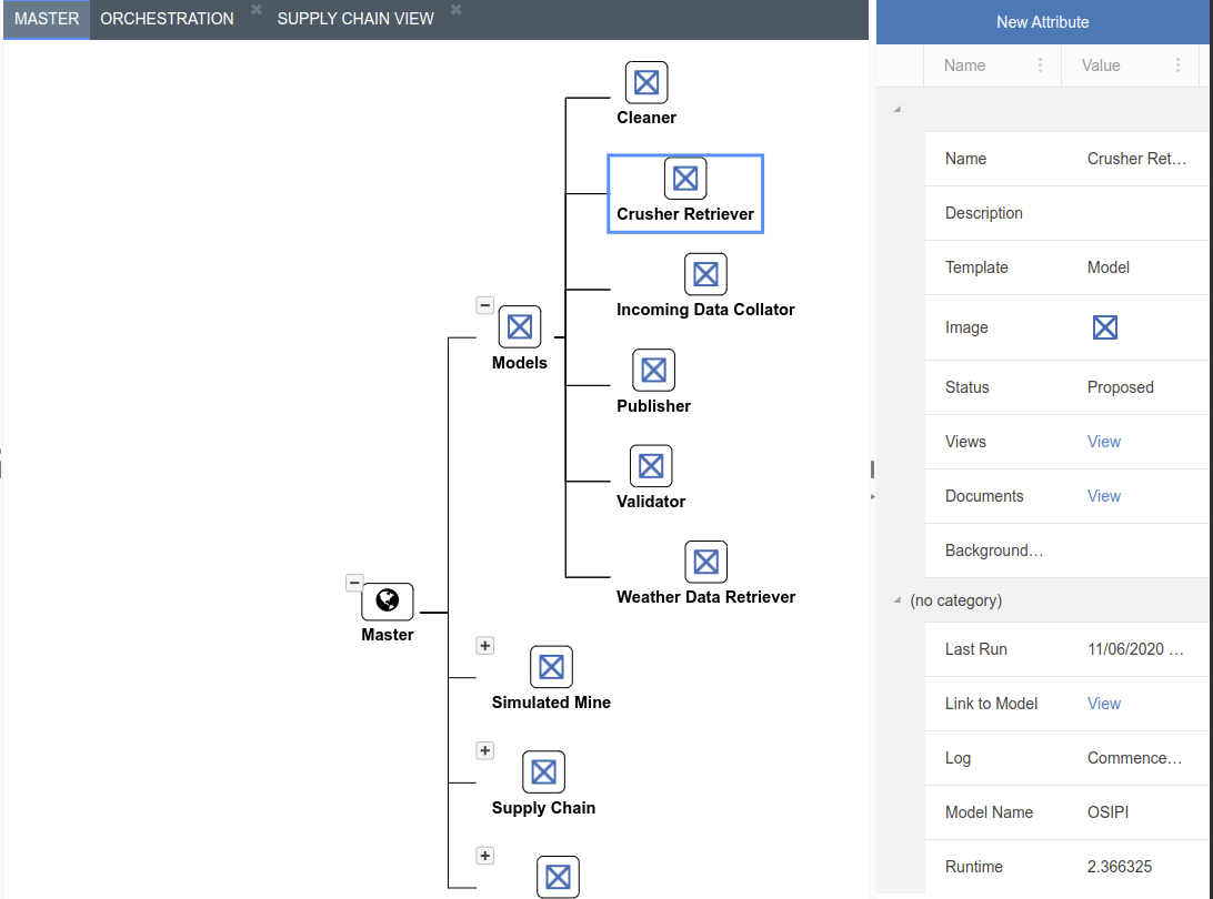
Move over to the Orchestration view, and drag/drop the assets onto the surface in the order they need to be executed.
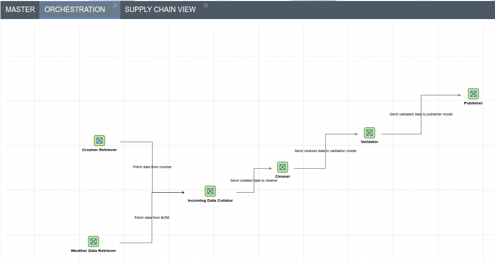
Once complete, run the orchestration model. The assets will change colour as the orchestration model is executed, blue to indicate running, green success and pink failure.
Also examine the asset attributes, they will include information such as the log, runtime etc.
Akumen’s Asset Library is a powerful tool for storing and contexualising data. As well as storing individual values such as numerics, text and dates against attributes of an asset, an individual attribute can be linked to a database tables, and filtered down to only retrieve data relevent to that asset. Database tables can be created as a result of standard model outputs, or created through Akumen’s API in the v2\Database section (see Swagger).
This code example shows how to fetch weather station information from the asset library, then how to write updates to include the current temperature and gps coordinates back to each individual asset. An output table is generated with the last 72 hour observation history, which we will then use to create a link back to each asset. Note that we can create the link to the table through the Akumen UI, but we will do that programmatically as part of the weather model.
Finally we will write a second Python model that retrieves data from the weather output table, filtering the data for the weather station we want to access the data for. The filter information is stored against the weather station’s attributes.
The assets we need to build need to be of template type Weather Station (see here for information regarding templates). Each weather station needs the following attributes for the following model to work:
| Attribute | Data Type |
|---|---|
| BOM_Id | Text |
| Current Temperature | Decimal Number |
| Last Updated | Text |
| Latitude | Decimal Number |
| Longitude | Decimal Number |
| Observations | Database Table |
| WMO | Whole Number |
Once the template is created, create 3 assets using this template called Jandakot, Perth and Perth AP. Note that we do not need to fill in all of the attributes, only enough for the model to populate them from BOM. For each asset, configure the follow (sourced from BOM):
Once the assets are built, create a new Python model called Weather Loader, replace the contents of main.py with the following code and execute the model. Once the model is executed successfull, you will notice that the rest of the attributes for the assets are populated. Running the model a number of times updates the values. Temperature, for example, contains the latest value, but the history shows the historical values. Also note the Observations database table - clicking on View should display a popup window with the data filtered on the currently selected asset. We will use this configuration in the next section to fetch data from the table to use in a new Python model.
The consumer model is simple in that it’s sole job is to fetch the assets from the asset library to retrieve the configuration of the database table attribute, and use that to fetch the data from the database table. Create a Python model called Consumer and replace main.py with the following code.
Basically this model will construct a dataframe from a data table in another model, using the configuration specified against an asset. The results are returned to the data tab
The following code example is similar to the previous weather example, except rather than just getting the historical values and populating the asset library, it uses Facebook’s Prophet Python library to use the incoming historical data to make a prediction on the future temperatures, creating some charts in the process.
By default, Akumen does not include the fbprophet Python package. Simply running the code below will return an error. We can create a file called Dockerfile. A template is created inside Akumen - simply add the line
to the Dockerfile. When the model runs, it will download and install fbprophet into the container your model runs in, and allows you to use that package.
Create a new Python model, and copy and paste the code below over the top of main.py.
Once the model has been run successfully, click the images button to see the generated images from the model, including the forecast trend and range of the forecast.
Datasource inputs are used to pass data from datasources into a Python application. Unlike Value Driver Model datasource inputs, a date column does not need to be specified.
Datasource inputs are created in Python by specifying a variable as a datasource:
The datasource is referenced on the research grid by right-clicking the datasource input and clicking “Select Datasource”. Doing this will open the following window:
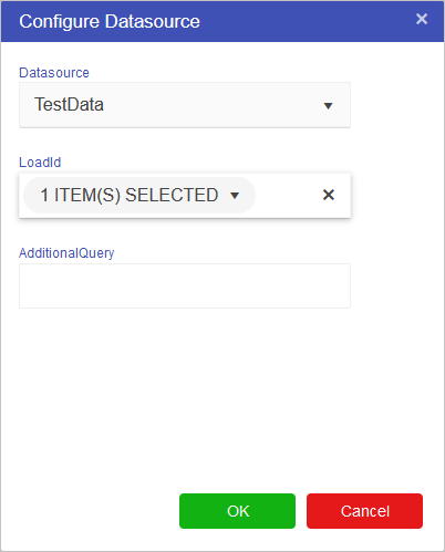
Only the “Datasource” field is required. Both the “Load ID” and “Additional Query” fields are optional. More than one Load ID can be specified, with the data filtered by that Load ID.
Datasource variables use a Pandas dataframe which can then be cleaned (if required) and processed.
For Python models built in Akumen, it is possible to change the Python image being used to another image that we host in Docker. There are some situations where you may want to do this, such as if you want your model to run with a different Python version.
The Python image can be changed through the model’s properties and is specified using the ExecutionImage key.
Where the ExecutionImage key is not provided, the 3.7.2 image is used so as to not potentially break existing Python models.
Python v3.7 is outdated and no longer supported by Python.
The 3.7.2 image is thus deprecated in Akumen and will be removed at a future date.
When this task is performed, models without the ExecutionImage key will default to using the latest image supported by Akumen.
If you wish to continue using the deprecated image after this time, please contact the Akumen support team to discuss your needs.
Changing the Python image can be done as follows:
ExecutionImage key will appear as shown in the image below
ExecutionImage key does not exist, it can be manually added by typing into the window. Note that this window is in JSON format and requires that a comma is added to the previous line as shown in the image.3.12-main is specified. Thus the entire line for the Execution image is: "ExecutionImage": "3.12-main"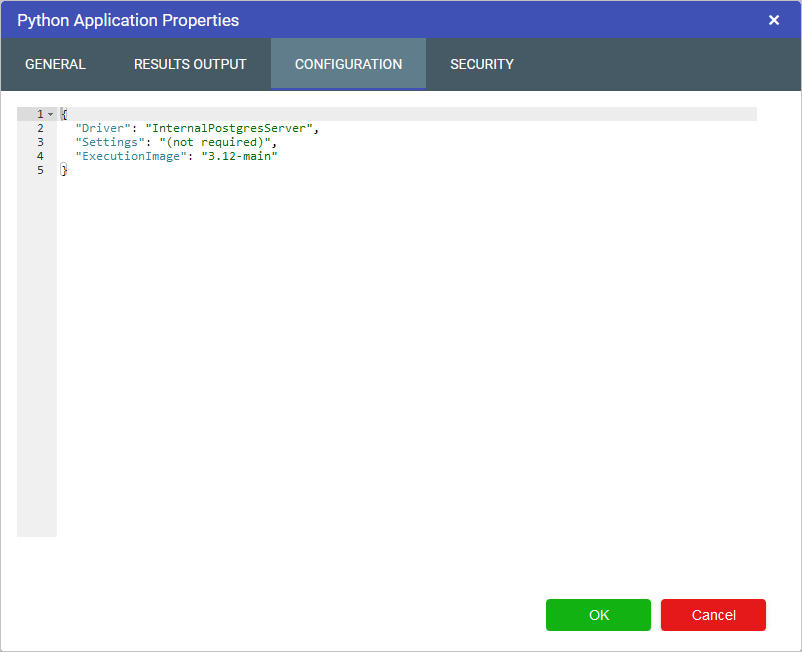
The Python packages supported in the “3.12-main” Python image are listed below.
| Akumen Message | Issue | Solution |
|---|---|---|
| Invalid setting in the model configuration for ExecutionImage | String entered is null or empty | Provide correct Python image name (e.g. 3.12-main). See image above. |
| You are using deprecated execution image. Consider switching to a supported image version | An earlier version (e.g v3.7.2) is being used or “ExecutionImage” is not specified in the model configuration | Use a later Python image version that is not deprecated (e.g. 3.12-main). See image above. |
| The container this model was running in could not find image | The Python image could not be found | Ensure that the Python image name is entered correctly (e.g. 3.12-main). See image above. |
Two of Akumen’s key capabilities are scenario flexing and scenario management, which can be handled in the Research tab.
Scenario flexing allows you to generate a number of scenarios based on altering individual parameter values. For example, you can create a number of scenarios, flexing the interest rate of an NPV model.
Scenario management allows you to clone, delete, reorder or baseline existing scenarios, along with manually altering parameter values for those scenarios.
These Scenarios allow us to look at the “What if…?” situations and plan for either
The research grid can be found by clicking on the Research button at the top right of the screen.

The research grid is where scenarios can be cloned and researched.

Below is an example of the different scenario parameters (columns) in the research grid.
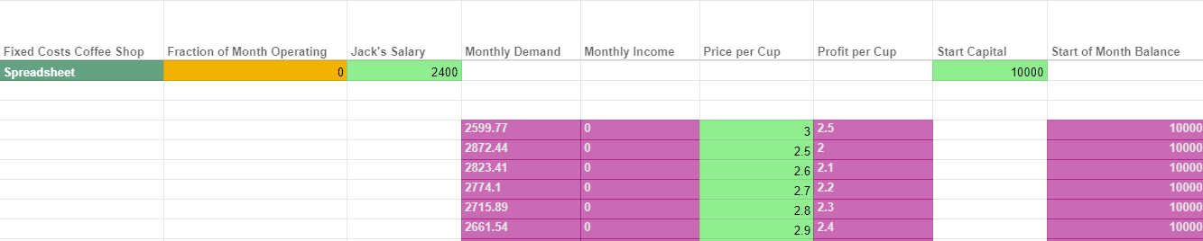
The rows on the grid are scenarios.
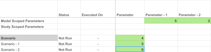
The research grid is broken up into a number of rows. Application Level Parameters are those parameters that affect the entire model, regardless of scenario. Think, for example, a carbon tax or life of mine. The second row is always the study level rows. These values can be altered on a study by study basis and apply to all scenarios within that study. All other rows are scenario level rows. These rows have individual values that affect only that scenario. Flexed parameters appear in these rows.
Right click options are available in this grid to perform tasks such as setting complex values (eg a tabular input) or performing scenario operations such as clone, delete or execute.
Once a model has been built, data added to it, then the real power of Akumen become visible. Akumen has the power to do advanced scenario analysis. This means that users have the power to investigate the “What if” questions. Lets say that in a model there are two inputs. If we wanted to change the second input but still see the results of the original value we could do something called cloning.
As the name suggests we can clone the model we have just built to adjust certain values and still see the results of both scenarios, the original and the clone, without rebuilding the model.
When building a Driver Model there are two ways to clone a scenario. You can clone them in the Driver Model Build screen or in the Research Grid. When using Python or R, you can only clone scenarios in the Research Grid.
Initally, in a new model or study, the top scenario will be the Baseline Scenario. Any scenario can become the Baseline Scenario by right clicking on the scneario and selecting Set as Baseline. Once set the scenario will be greyed out and the font made bold. The Baseline Scenario is the scenario that we recommend cloning scenarios from as it should contain the default parameter values for the entire study.
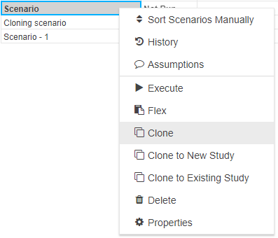
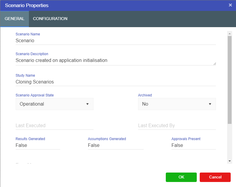
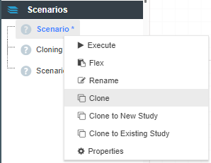
Parameter scoping is how the value of parameter affects other scenarios within the model. There are three levels of scope:
As you can see in the image above, there are two parameters at the model level, and one at the scenario level. Changing Parameter - 1 from 5 to another value in the top row means that value is applied to every scenario. Parameter is set at the scenario level, where each value is different across each scenario.
Flexing is often the best way to answer the “What if” question for fixed input values in your model.
Flexing creates a range of scenarios using the specified start value, final value and a step value which determines the increment used.
There are two methods available for users to flex inputs.
From the scenario list:
There is a hard limit to the number of scenarios that can be flexed. This is displayed in the flexed scenario window.
From a fixed value input node:
It is possible to have multiple nodes selected on the driver model canvas when opening the flex window using this method. If this is done, each input parameter node selected will be added to the flexing grid.
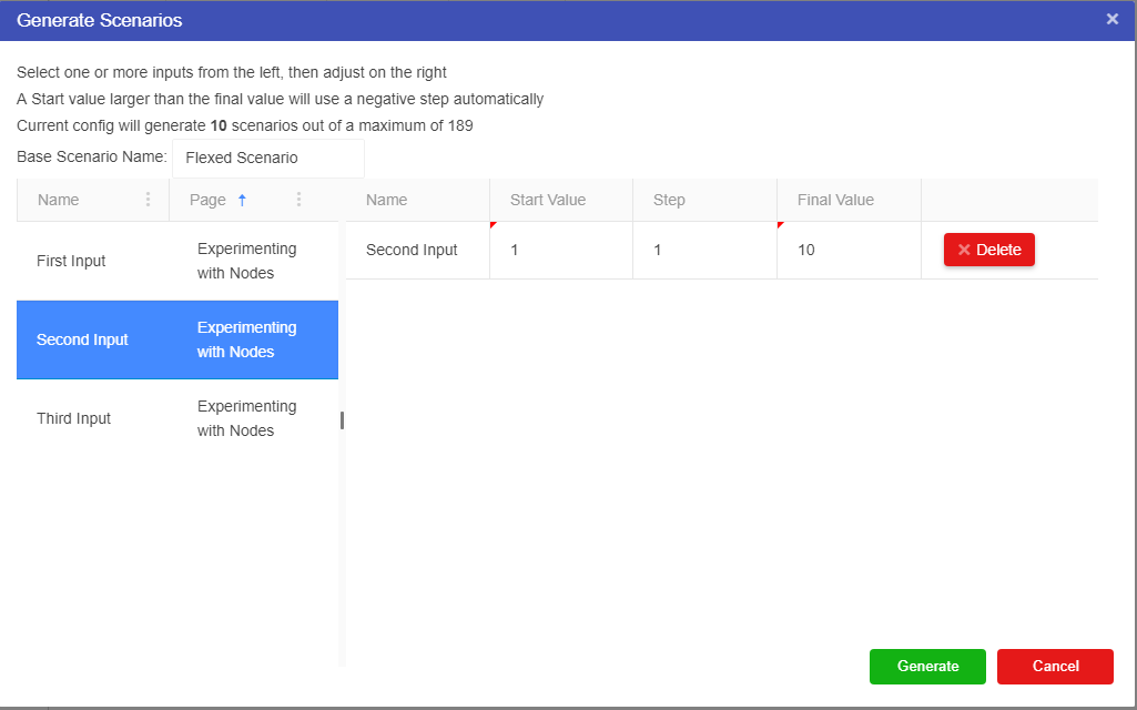
Flexing can be performed for more than one input at a time. For example, you could flex one input and then a second input at the same time with the same values. The model will create these scenarios as long as it has not reached the limit of scenarios that it can generate.
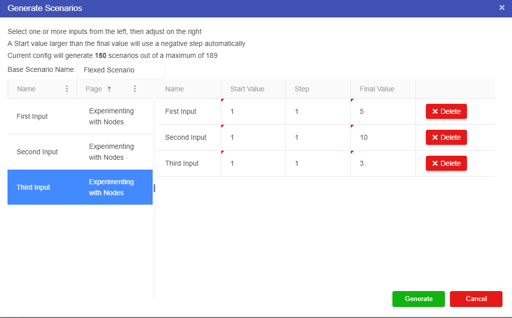
Once you have created the scenarios that you want to investigate you will need to execute them to view the results. You can either execute a single scenario, a range of scenarios, or all the scenarios in a study.
To execute a single scenario:
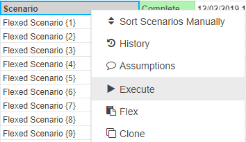
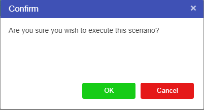

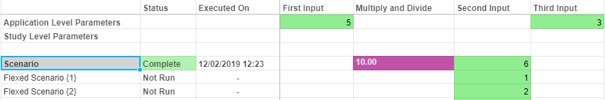
To execute a range of scenarios:
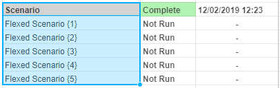
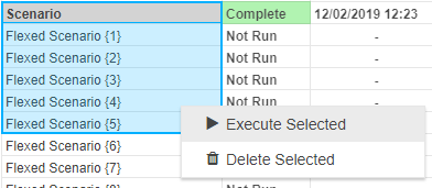
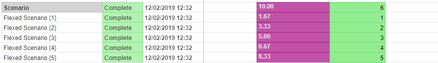
To execute all the scenarios in a study:

To view logs:
All model types record logs of their execution. In addition, adding print (or progress) calls in your code will include those statements in the run log. Right click on the scenario and click Logs to access the latest run log. In Py and R, it can also be accessed below the code editor using the Logs button.
To view run log history:
Run log history is also retained for each scenario, up to a maximum of 50 runs. Akumen will remove older logs outside the limit of 50. In addition to the history it stores the log file for that run. There is also an API call to access the run log information (see the API docs for access to the run log history). The url for this is /api/v2/models/{model_name}/execution_history
By default, Akumen ensures input and output consistency by resetting the run status and clearing all outputs of executed scenarios when a number of different events occur:
Sometimes, this may not be the desired behaviour, especially for applications that take a long time to generate outputs. There are two ways of preserving outputs in Akumen. The first is to simply use the application, study, scenario cloning capabilities in Akumen. However this does not enforce preservation of outputs. It is up to the user (and/or security) to ensure outputs are not accidentally cleared when there is a change.
Output protection provides controls over what can be modified so outputs are not accidentally cleared by editing different parts of Akumen.
When an application is created, the application is created with output protection off. This means the behaviour listed above applies. An application can have it’s output protection toggled through Application Properties.
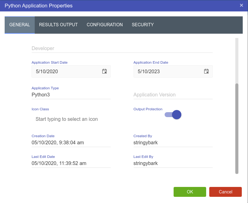
It can also be toggled in the model through the toggle next to the model name.
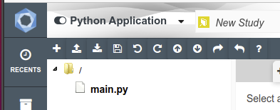
Output Protection status is shown by a toggle in the application manager.
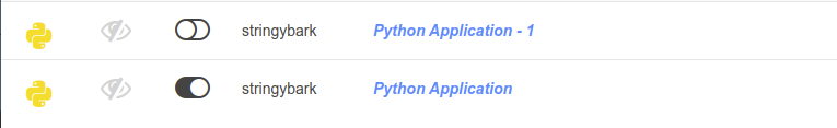
Output protection changes the above behaviour as follows:
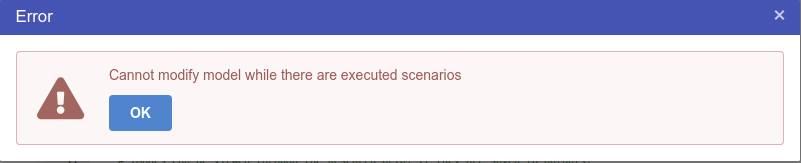
Scenarios, Studies and Applications can have their outputs cleared and run status reset so they can be edited. This is a manual process through right click on the research grid, or through the Model or Study dropdown above the research grid. Once the scenario outputs are cleared, the operation can be retried.
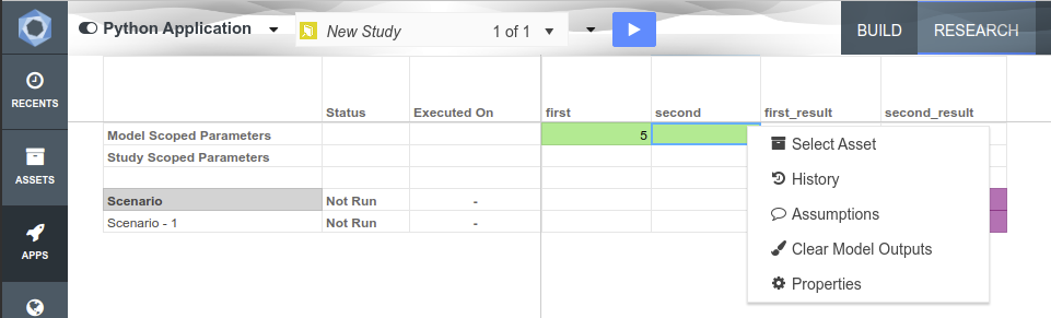
Akumen has the potential to create hundreds of scenarios, each representing a what-if question in your model. With all these scenarios being created, it is important for users to understand how to group scenarios so that they don’t get lost. The best way to do this is through the use of Studies.
At the top of any Application there will be a dropdown menu with study written at the top (See below).

By using the dropdown menu users can sort and organize the different scenarios that have been created by cloning or flexing. Studies also allow for certain values to be used across the entire study or across all studies for ease of evaluating the best scenario to use.
To create a new study:
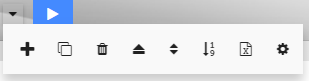
When a new study is created the baseline scenario in the original study is carried through into the New Study and becomes the new study’s baseline scenario. Once a new study has been created users can rename the new study. It is always recommended that different Studies be given unique names that allow users to identify which study is which, and what types of scenarios they can expect to find in each study.
To rename a study:
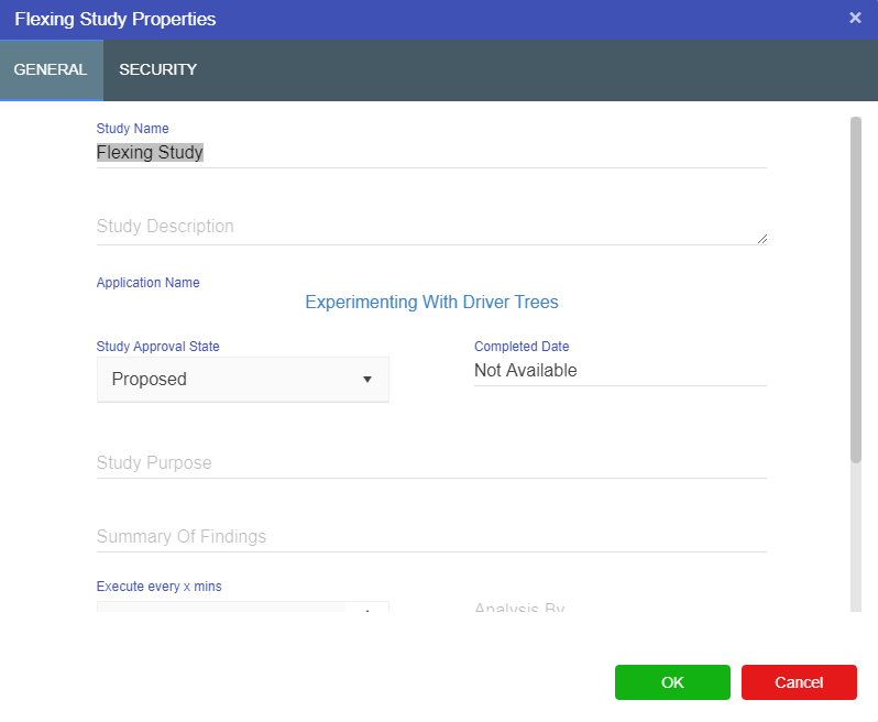
Study Functions:
The study functions available through the dropdown include:
Once a scenario, study, or application has been executed the raw data is sent to the Data tab. The Data tab allows users to preview an query the raw results of any scenarios that have run without returning an error. This functionality works in the same way regardless of the language (Driver Models, Python or R) that is used. If a scenario runs but returns an error there will be no data to display for that scenario.
The Data screen is broken up into two sections:
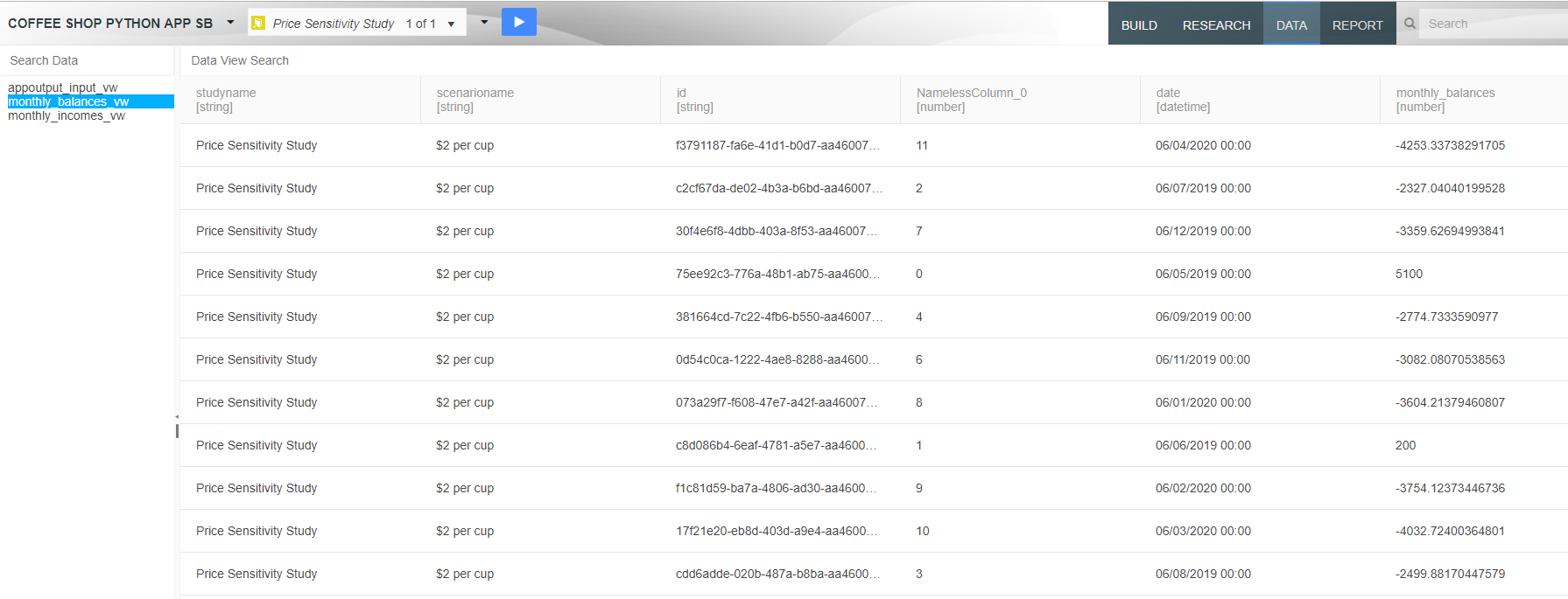
Selecting one of the available data tables in the list will display the data in that table (when users first open the data tab the data table will be empty). This list will vary depending on what tables are generated by the application. These tables support the following functionality:
To access any of these functionalities simply right click on data table in the list and select from the displayed options.
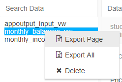
When exporting the whole table be aware that this can cause issues with browsers if there is a lot of data in that particular data set. If a user reruns the application than the data tables will be recreated. By exporting tables users can import these data tables into other models in Akumen manually, however these data tables can also be directly imported into other models.
When a data table is selected from the list the data stored in that table is displayed. These entries can be:
Data is sorted by column. To sort the available users only need to click on the column they want to sort by. For number columns the sorting starts from 0 and goes to the maximum number. For strings, the sorting goes A-Z. Each column also displays the datatype the data is stored under. This is useful when diagnosing reporting issues and data type errors.
The Data View Search box allows the user to search the data set, using a Sql like syntax, eg "scenarioname"='Scenario' will filter on the scenario called Scenario. Note we enclose the scenarioname column name in double quotes. This is because there is the possibility that columns are case sensitive, and double quotes are required to enforce the case sensitivity in the database engine.
Whenever a user runs scenarios in an application and and those scenarios return as complete the results are sent to the Data tab. Any table in the data tab are automatically available in the reports.
Akumen’s reports provide an interactive results dashboard where users can create graphs and other visuals in order to view their model’s results.
However the process of creating reports for Driver Model and creating reports for Python and R vary.
To access Driver Model results users need to ensure that the tick-box in the properties box of each node which says Publish to Results has been selected. If that box has not been selected then there will be no results for the query to draw from.
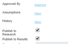 . An chart icon will appear on the node indicating it is published to results.
 ![]()
![]()
For Python and R users there needs to be a specified output in the return {} or ret() section of the code. If there is no output specified then there will be no data for the reports to draw from.
For more on how to create Reports for both Driver Models, Python, and see the Reports section.
How to take model results and turn them into informative visuals.
Once a scenario has run users can use the scenario results to populate a report.
Reports can be accessed one of two ways:
We recommend that when users are going to create new reports that they create them via the reports tab in their applications since this way the application can give users the correct set of reports that can be created for that model.
Creating reports for Driver Models differs from creating reports for Python or R models. However finding the Report tab in models remains the same.
In any application there are 4 tabs:
Reports are stored in the Report tab, and model results can only be accessed if scenarios have been executed and returned Complete. Only values that have been specified as outputs will be available for use in reports.
All model types will need to have specified outputs in their code or properties for any outputs to successfully be recorded for use in reporting. For Python and R the outputs will need to be specified in a specified output in the return {} or ret() section of the code. For Driver Models, each node as a tick box in the properties that says Publish to Results. If this box is not ticked their will be no specified output for the Driver Models and therefore there will be no results to use for in the reports.
For Driver Model, Python, and R users there is an option to add an External (URL) Report to the Reports section. This allows users to use data from executed scenarios and populate any external reports that users may be using already.
To set up an External Report:
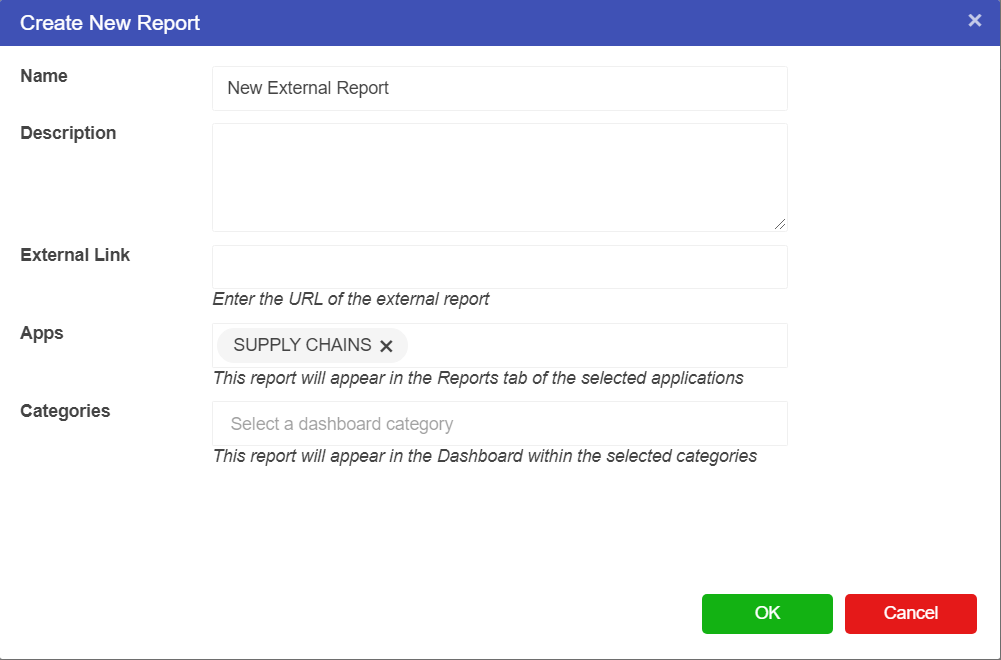
You will then be taken to the reports screen and the URL given when the report was set up will be embedded into the reports screen.
Need a user interface for your Application? Or do you just want to render another system’s web page within Akumen? Akumen pages are your answer.
There are 3 types of Pages that can be created in Akumen’s Page Manager:
Users can select any one of these to create and one three types of Pages.
A Blank Page is like a blank canvas. Users are starting the page build from scratch. It is intended that these pages are only used by those who are familiar and experienced building webpages since Pages is a link to create embedded pages over the top of working models.
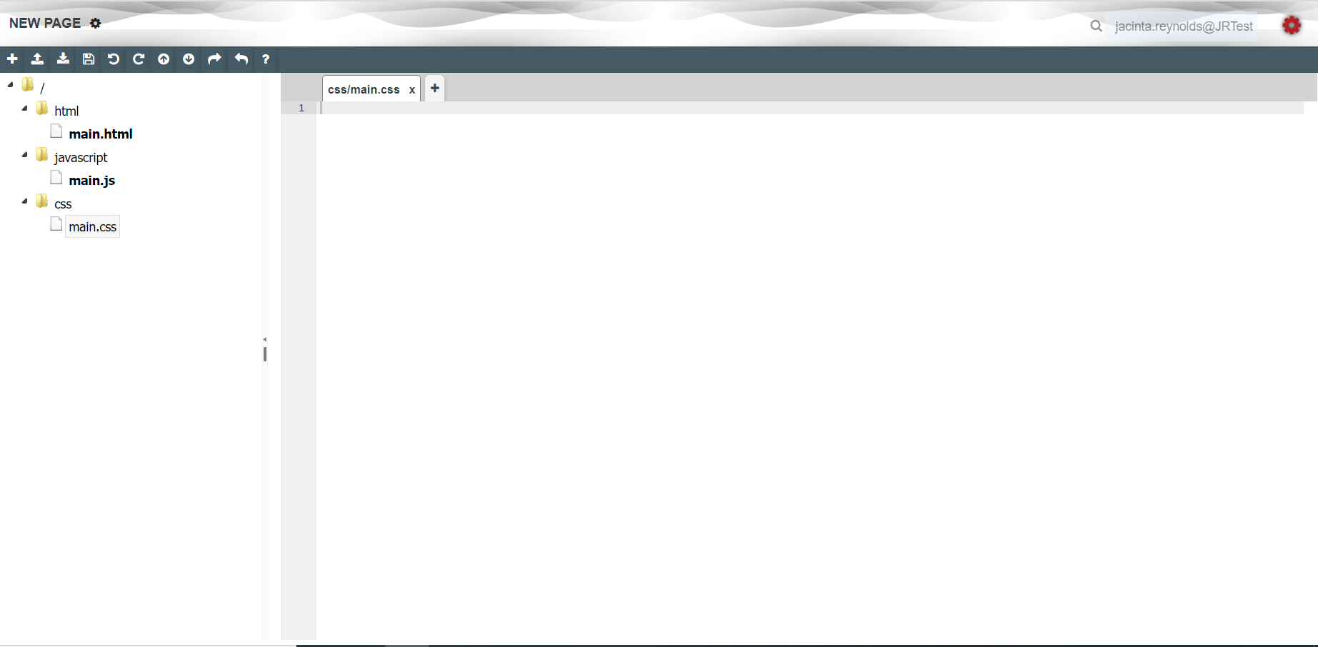
A Template Page creates a Page template upon creation. It creates all the necessary javascript and html needed for the page to run as long as it is linked to an application. To link it to the application simply select which model you want to connect the Page to from the avilable models.
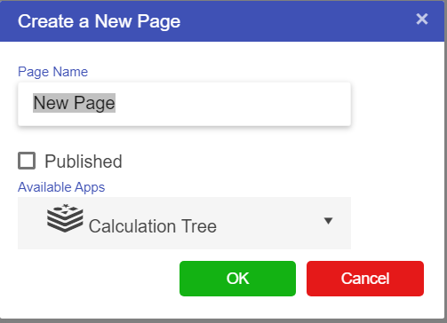
Once connected the page will create a fully useable starting point for a fully functioning interactive page.
An iFrame Page is like pointing the page in the direction of an external page and can render any external page, as long as users have the URL. Some sites like Google prevent embedding their sites in an iFrame. If a page doesn’t display, you will need to access the Chrome developer console to check any errors. The following error will appear if a page is not available to embed in an iFrame.

The Page Manager (accessible through the Pages menu item in the navigation bar) shows all the pages you have permissions to access.
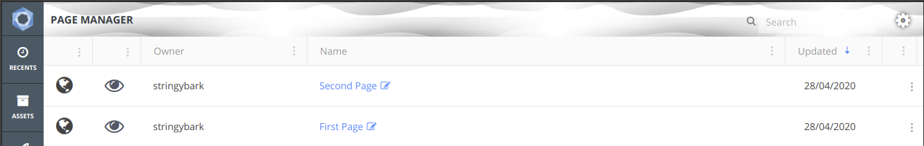
Clicking on the page takes you to the rendered page output, as shown in the template example below. If you have permissions to edit the page, an Edit icon appears next to the title as shown in the page manager above.
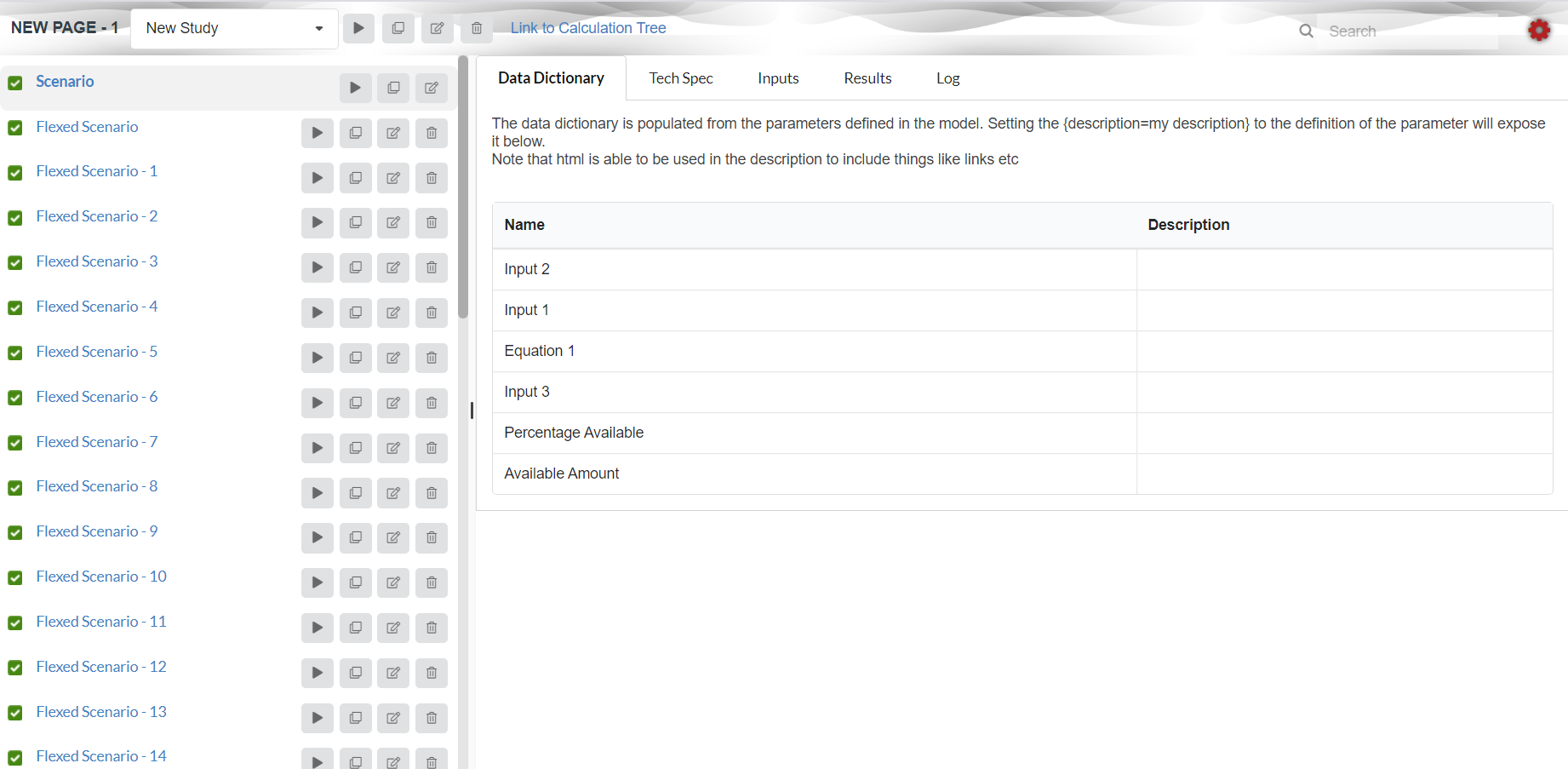
Pages are Akumen’s customisable UI’s. They can be built using HTML, JavaScript, and CSS.
Any number of files can be created in the page’s directory structure. This can be performed by clicking the + button in the toolbar as shown in the image below.
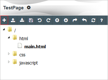
Folders can be created in the directory structure by specifying a path in the file name when creating a new file (e.g. folder_name/test.html).
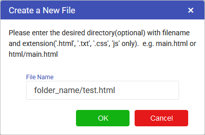
To specify the main entry point for Akumen, one of the HTML files must be specified as the startup file. By default, the first HTML file created is set as the startup file. The startup file can be changed to a more suitable file by right-clicking a HTML file and selecting “Set as startup file”.
JavaScript files are always loaded into the browser, however HTML and image files are not loaded with the exception of the startup file.
To include other HTML files, create a <div id="tech_spec"></div> element with an id, and use the attachHtmlToDiv inbuilt JavaScript function to attach the JavaScript file.
For example, to attach the html/tech_spec.html file, use the following code
Akumen API documentation is available by accessing the Cog in Akumen, then clicking Help, API Docs. A limited number of “convenience” functions have been created to reduce the time taken to create pages in Akumen, documented below.
| Name | Description |
|---|---|
| apiToken | The api token key used to provide access to the Akumen API. Key is set based on the currently logged in user, not the user that created this page. |
| userName | The currently logged in user, which can be used for some notification interactions |
| clientName | The current client name, which can be used to automate API calls when switching between clients in the same Akumen instance |
There is a javascript dictionary available with the Page configuration (set through properties) called configuration. For example, if the scenario configuration is set to {"test":"test"}, use javascript to get configuration["test"]
To support linking a “templated” external page to an application (with a selected application), there are some configuration parameters available, set through the properties of the page
akumenApi(apiPath, type, data, callbackFunction, errorCallbackFunction, api_version)
Constructs an AJAX call to the Akumen API, optionally executing the callback function with any returned data
akumenFetchApi(apiPath, type, data, callbackFunction, errorCallbackFunction, api_version)
Constructs a fetch api call to the Akumen API, optionally executing the callback function with any returned data
In addition to the above call to access the API, there are a number of “convenience” functions to provide easy access to Akumen"s API. All support a callbackFunction in the event of a successful API call. For each of the calls below there is the base call, and a fetch api call, just append Fetch to the function name For example, getModel would also have a getModelFetch call.
getModel(modelName, callbackFunction, errorCallbackFunction)
Gets an Akumen model by name, including it"s studies, scenarios and parameters
getStudy(modelName, studyName, callbackFunction, errorCallbackFunction)
Gets an Akumen study by name including it"s scenario
getScenario(modelName, studyName, scenarioName callbackFunction, errorCallbackFunction)
Gets an Akumen scenario by name
getInputParameters(modelName, studyName, scenarioName, callbackFunction, errorCallbackFunction)
Gets all the input parameters associated with a particular scenario
saveInputParameters(modelName, studyName, scenarioName, inputParameters, callbackFunction, scope, reset_run_status, errorCallbackFunction)
Save the array of input parameters, optionally setting the scope and resetting the run status.
saveInputParameter(modelName, studyName, scenarioName, inputParameter, callbackFunction, scope, reset_run_status, errorCallbackFunction)
Save an individual input parameter, optionally setting the scope and resetting the run status.
cloneStudy(modelName, studyName, callbackFunction, errorCallbackFunction)
Clones a study, including all it"s scenarios, inputs etc
deleteStudy(modelName, studyName, callbackFunction, errorCallbackFunction)
Deletes a study and all of it"s related data
cloneScenario(modelName, studyName, scenarioName, callbackFunction, errorCallbackFunction)
Clones a scenario, and all of it"s inputs
deleteScenario(modelName, studyName, scenarioName, callbackFunction, errorCallbackFunction)
Deletes a scenario and all of it"s related data
createRequiredFieldValidator(container, message)
Creates an instance of a required field validator, attached to the container jquery object. Also sets the message
executeStudy(modelName, studyName, scenarioNames)
Executes a given study in a model, optionally passing in a list of scenarios that can be executed within the study
execute(modelName, inputParameters, callbackFunction)
Executes a model with the given list of inputParameters
getViews(modelName, callbackFunction, errorCallbackFunction)
Get the views created as part of an R or Python execution
getResults(modelName, studyName, viewName, query, sorts, fields, callbackFunction)
Gets the results for the study and view, passing through the appropriate query, sorts and fields.
getOutputs(modelName, studyName, scenarioName, callbackFunction)
Gets Akumen internal outputs for the given scenario, such as those available in Akumen Internal Reporting
getRoles(callbackFunction, errorCallbackFunction)
Gets the list of rolenames the user belongs to. This allows the page developer to customise the page based on role name.
There are additional html functions to be able to attach additional HTML and Image files to the page
attachHtmlToDiv(filePath, div)
attachImageToDiv(filePath, div)
Popup notifications popup a small notification in the bottom right corner
NotifyPopupDefault(message)
NotifyPopupSuccess(message)
NotifyPopupError(message)
NotifyPopupWarning(message)
progressIndicator(state)
Displays a progress indicator on the screen. Must be turned on by passing in true, and off by passing in false after asynchronous calls have completed
Akumen provides a number of notifications that can be subscribed to, using the function below.
subscribeToEvent(eventName, callbackFunction)
Subscribes to one of Akumen"s notifications
Additionally, a number of “convenience” notification functions are available to subscribe to. These require access to the ModelId, which can be fetched using the getModel(…) API call
subscribeToStudyExecutionCommenced(modelId, callbackFunction)
Occurs when execution of a study in the model commences. Returns the StudyId of the study that was commenced
subscribeToStudyExecutionComplete(modelId, callbackFunction)
Occurs when execution of a study in the model completes. Returns the StudyId of the study that was completed
subscribeToScenarioCollectionChange(modelId, callbackFunction)
Occurs when the scenario/study collection of a model is changed (eg new scenarios, scenarios updated etc)
subscribeToGeneralMessage(modelId, callbackFunction)
Occurs when a general message from execution of a model occurs
subscribeToGeneralError(modelId, callbackFunction)
Occurs when a general error occurs during execution
subscribeToInputParameterChange(modelId, callbackFunction)
Occurs when a change is made to input parameters for a model
subscribeToDatabaseTableInserted(table, callbackFunction)
Occurs when data is inserted via API call to the specified table
subscribeToDatabaseTableUpdated(table, callbackFunction)
Occurs when data is updated via API call in the specified table
subscribeToDatabaseTableDeleted(table, callbackFunction)
Occurs when data is deleted via API call from the specified table
Although any javascript package that is available through CDN (Content Delivery Networks) can be used by Akumen’s Pages, this is generally not recommended in a production environment due to the possibility of the CDN not being available. Examples of CDNs include jsdelivr or cdnjs.
Akumen provides minified versions of some of the more common packages including grids and charts. They only need to be included in on of the html files in your project, using the following syntax:
<script src="/bundles/vue.js"> or <link rel="stylesheet" href="/bundles/buefy.css" />
This includes the Vue framework, including Semantic UI Vue as well as a date picker control for Vue.
Packages include:
Utilising the bundles means that Akumen can fetch the bundles locally, instead of fetching them from remote sources.
If further bundles are required, contact Akumen Support to include them in the release.
In addition, bundles and other libraries can also be included in the main page load using configuration on the page itself. This provides a better experience in that these bundles are loaded prior to the user specified page loading. See here for more information.
There are some cases where pages are built to suit low end devices, such as iPads on the factory floor that cannot handle Akumen’s full suite of Javascript, and do not require Akumen’s navigation side bar and header. The integration page outlines the “Minimal” flag which tells Akumen not to load all it’s surrounding javascript.
Manage document and file uploads for use in applications and assets.
Akumen has the ability to store files and documents for use in applications and the Asset Library. Users can upload many different file types into Document Manager. Some examples of acceptable files are as follows:
With Excel files it is important to note that only .xlsx and .csv files can be uploaded into Akumen for use in applications, otherwise there might be errors with the inputs when the xlsx files are uploaded into the spreadsheet cells. Macro enabled workbooks are generally not supported.
As you can see in the list above the Document Manager simply stores the documents and makes them available for other users to use and attach to assets and use in applications.
Only Builders and Administrators can upload files and download them from the Document Manager. If you are a user and you cannot find a particular file then it would be best to contact a Builder or Administrator and get them to upload the file for you.
To upload a file to the Document Manager:


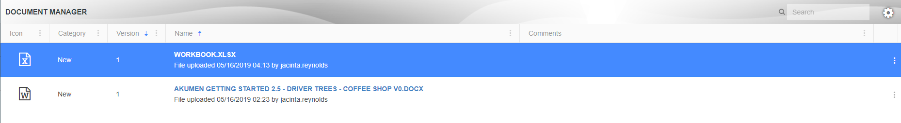
At the end of each upload are three dots. If you click on them the options menu for each uploaded file will appear. This will give you access to the file’s properties where you can attach comments about the file, but it will also allow those with permission, the ability to:
Documents and files that are uploaded ot the Document Manager can be attached to various Assets and Applications. There are two ways to link a document to an Asset or to an Application.
To upload a document:
To an Asset:
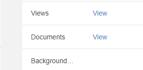
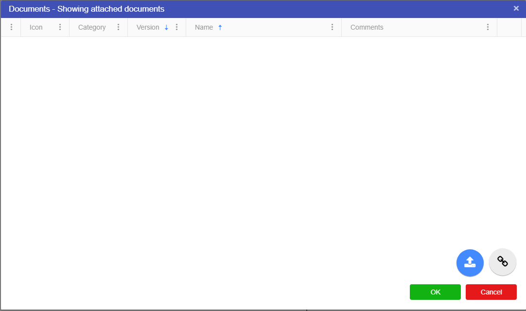
To an Application:
The process for linking a document from the Document Manager to both an Asset and an Application is the same as above except instead of clicking on the uploads button click on the link button. This will bring up a list of the documents in the document manager. By selecting any one of the documents in the list you can link them to your Asset or Application.

Akumen includes a rich set of API functions to allow programmatic access to Akumen. It is protected through an authentication token, where each user has their own resettable unique key. APIs can be used internally, for example through model execution or pages, or for third party tools and systems to access and update data stored in Akumen.
API calls are case-sensitive! Make sure to double-check to avoid errors!
To find this list of API docs:
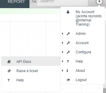
This chapter covers security configuration.
Akumen supports two modes of authentication - internal and OIDC (Open ID Connect). By default your tenancy will be set up with internal authentication - a username and password handled by Akumen.
Open ID Connect is a standardised extension of the OAuth 2.0 protocol which is used for authentication and authorisation. The Akumen Support team can configure OIDC against your tenancy, or it can be configured by an admin from within your own client. This is detailed in the OIDC Authentication section.
To access the configuration, navigate to the My Client option in the right hand cog menu, shown in the screen capture below
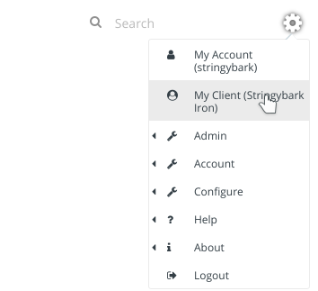
Click the Authentication Settings button to open up the settings window.
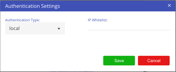
The default is local for local authentication, and an empty whitelist. See IP Whitelisting for how to configure IP Whitelisting for your client.
To configure OIDC, a number of steps are required. This includes both Akumen configuration and configuration of the OIDC provider. This guide steps through setting up common providers such as Azure and Google.
To setup OIDC, change the authentication type to OIDC, as shown below.
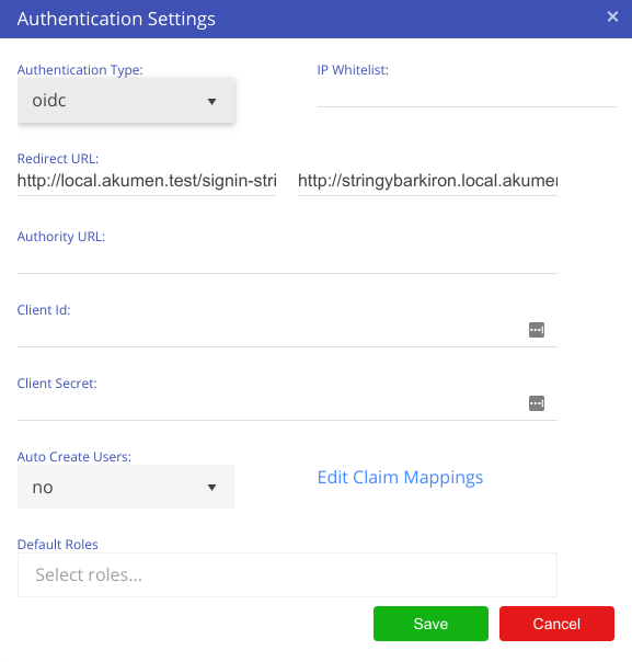
| Name | Description |
|---|---|
| Redirect URL | The redirect URL is a unique generated URL, and is unique throughout the Akumen system. There are two generated: The first is for the standard Akumen URL, the second is for future use where the tenancy name can be used as part of the URL. |
| Authority URL | The authority URL is the URL used to authenticate Akumen against. That is, the OIDC provider’s authentication URL. |
| Client Id | This is also the “application id”, that is the unique id provided to you from the provider to allow Akumen to authenticate against that provider. |
| Client Secret | A client secret can be defined on the provider, but can also be left empty if the provider does not require one. For example, Google must have a secret, but Azure may or may not have one. |
| Auto Create Users | With this option enabled, if a user attempts to access Akumen, the user account will be automatically created, but marked as inactive. The user will not be able to login in until the administrator of the tenancy enables that account. |
| Default Roles | Where the provider does not include roles as part of claims (such as Google), the user can be automatically created with the selected role or roles. This is not used with providers that include roles as part of claims (such as Azure). |
| Edit Claim Mappings | Although OIDC is a standard, the claims that the providers can use is not. This provides a mapping of claims Akumen uses, mapped against the provider’s claims. Akumen already has default claim mappings for the three providers Google, Azure and AWS, though they can be edited if required. |
When logging into a client using OIDC, a username is not required. Simply enter @TenancyName into the username box where “TenancyName” is the name of the tenancy you are logging in to.
The password field will disappear once you hit enter or tab out of the username box. If everything has been configured correctly, you will be redirected to your OIDC provider to authenticate against.
Once authenticated, you will be logged into Akumen.
The Akumen user account’s email address is required to either be a match of the OIDC provider’s email address (e.g. Azure, Google) or a plus addressed form of it.
In the former method, if the user’s Azure email address is first.last@company.com, then the user’s Akumen email address must also be set to first.last@company.com.
In the latter method, plus addressing needs to be specified for the user’s Akumen email address. This may be done when a user needs SSO for multiple tenancies in the same Akumen environment.
If using plus addressing, the format of the user’s Akumen email address will need to appear as first.last+tenancyname@company.com.
The Akumen username must also match everything before the @ character in the OIDC provider email address.
For example, if the email address retrieved from Azure is first.last@company.com, then the username must be specified in Akumen as first.last.
Also, the Akumen email address without the plus addressed section must match the OIDC provider email address.
For example, if the email address retrieved from Azure is first.last@company.com, the email specified in Akumen can be first.last+tenancyname@company.com but cannot be firsty.last+tenancyname@company.com.
When users are created automatically, they are in effect linked to the OIDC provider via the email address. This way, any users already in an Akumen tenancy can be converted from a local user to an OIDC user by simply ensuring the email address matches the OIDC provider’s email address, and setting the IsExternallyAuthenticated flag to true (note that this flag is only available for OIDC clients).
This also means that users can be created without the flag set, meaning an admin user for the tenancy can still login without being authenticated against the OIDC provider.
Where roles are returned from the OIDC as claims, and the user attempts to login, all role membership for that user are cleared from Akumen. Akumen then looks at the Auth Group Name field in the role to attempt to match the claim with an Akumen role. If the returned claim matches an Akumen role via the Auth Group Name field, the user is then added to the role. If no roles are configured, the user will be denied access to Akumen.
If there are no roles returned in the claims by the provider (eg Google), Akumen will use it’s own internal roles.
Azure setup involves logging into Azure, accessing Azure Active Directory, then App Registrations.
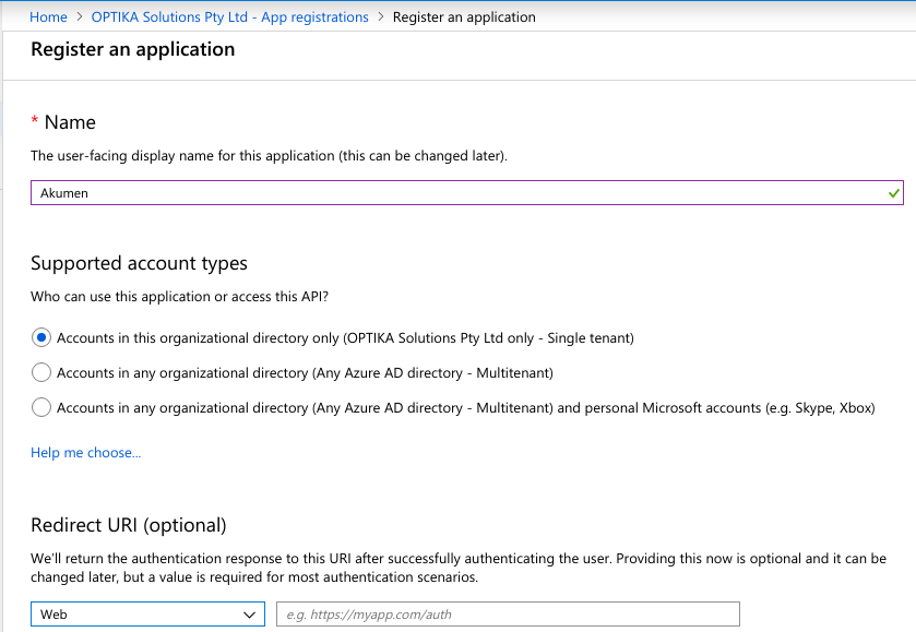
https://login.microsoftonline.com/, followed by the “Directory (tenant) ID” from Azure.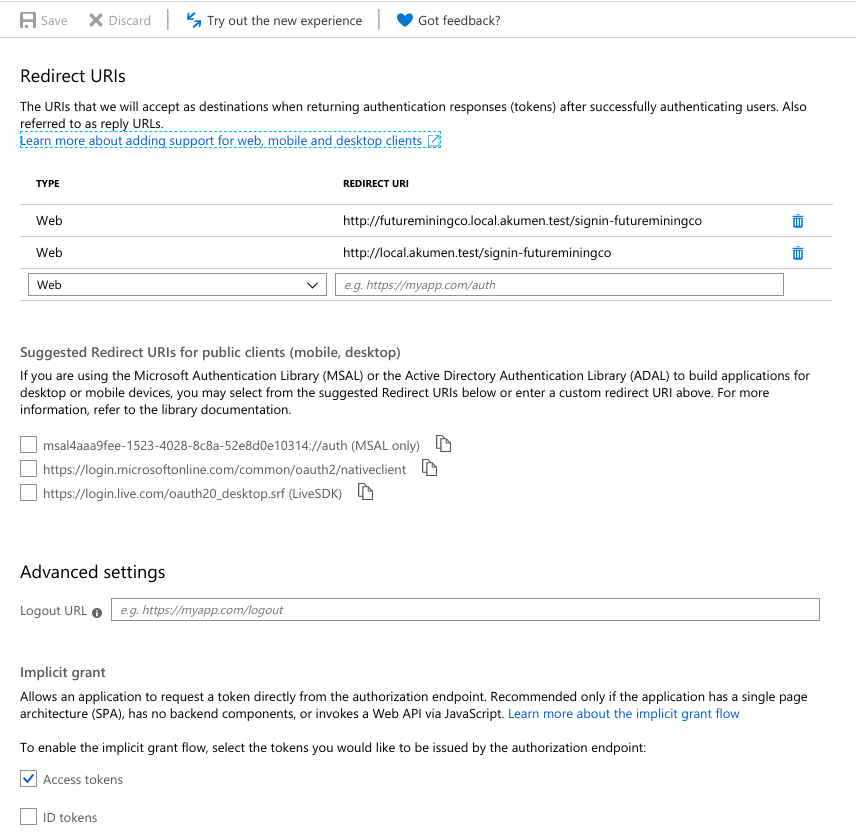
To configure Azure AD to pass AD group memberships as claims to Akumen, edit the manifest and replace "groupMembershipClaims": null, with "groupMembershipClaims": "SecurityGroup",.
To map each AD group to an Akumen role, copy that group’s Object Id from the Groups section of Azure Active Directory, then enter that Object Id as the Auth Group Name of the matching Akumen role.
Google setup is generally only used for a single user account, rather than enterprise, but is listed here for completeness.
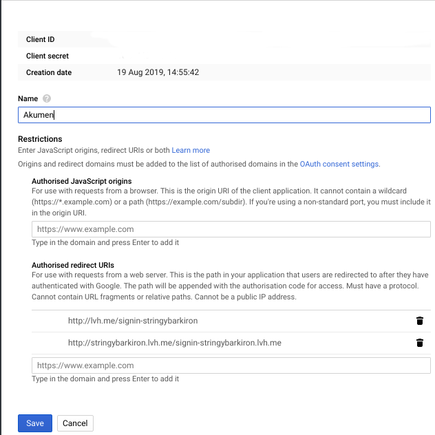
Clients can also set IP whitelists to ensure that their Akumen accounts can only be accessed from configured IP ranges. This is done through authentication settings, as described in the previous sections.
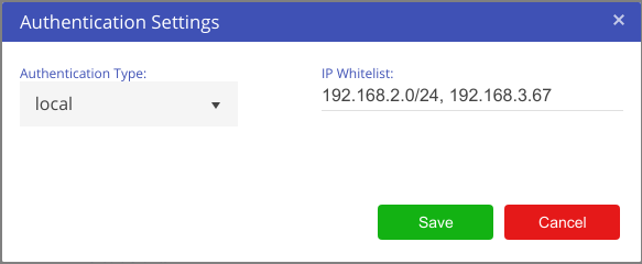
As seen in the above configuration, either a CIDR block or a specific IP address can be specified. IPv6 addresses and CIDR blocks can also be specified.
IP Whitelisting behaves slightly differently depending on local or OIDC authentication. In local mode, IP Whitelisting will simply prevent anyone from logging into your tenancy unless their ip address is whitelisted.
In OIDC mode, if Akumen detects the IP address is part of the whitelisted range, it will automatically authenticate you against the OIDC provider, providing there are no IP range clashes between your tenancy and another tenancy. In that case the normal login screen will appear, as Akumen cannot determine the appropriate client.
At Idoba, security is our absolute highest priority. Therefore we take myriad security measures to ensure that the data of our customers and pentesters is secure and safe. In the spirit of openness and transparency, here are some of the security measures we take to protect and defend the Akumen platform.
Idoba leverages Amazon Web Services Web Application Firewall (WAF) and AWS Shield to protect the site from:
Distributed denial of service (DDoS) attacks Blocking of suspicious activity SQL injection, comment spam Possibility of quickly blocking IPs or entire countries
All HTTP-traffic to Akumen runs over an SSL-encrypted connection and we only accept traffic on port 443. The status of our SSL configuration can be found here.
During a user agent’s (typically a web browser) first site visit, Akumen sends a Strict Transport Security Header (HSTS) to the user agent that ensures that all future requests should be made via HTTPS even if a link to Akumen is specified as HTTP. Cookies are also set with a secure flag.
Akumen is hosted via Kubernetes and managed within Amazon data centers that leverage secure Amazon Web Service (AWS) technology.
Akumen’s backend is supported by a Postgres database to persist data. All data at rest and associated keys are encrypted using the industry-standard AES-256 algorithm. Only once an authorised user is granted access to their data will that subset of data be decrypted. For further details around the encryption at rest please see AWS encryption procedures.
Static files, such as images and other documents are persisted using AWS S3 storage. All static files are encrypted before they’re stored so while at rest they are encrypted.
Akumen entirely resides on servers located within Australia, and all data is stored securely within Australia. In the event that this changes (e.g. for geo-distribution, performance or durability purposes), all clients will be notified ahead of time.
Amazon Web Services undergoes recurring assessments to ensure compliance with industry standards and continually manages risk. By using AWS as a data center operations provider, our data center operations are accredited by:
ISO 27001 SOC 1 and SOC 2/SSAE 16/ISAE 3402 (Previously SAS 70 Type II) PCI Level 1 FISMA Moderate Sarbanes-Oxley (SOX) More information about AWS security can be found here.
During an account creation and password update, Akumen requires a strong password that has 8 characters or more, and contains numbers as well as lower- and uppercase letters. We do not store user passwords: we only store one-way encrypted password hashes, including:
Following an email change, password change or similar sensitive user account changes occur, the user is always notified in order to quickly be able to respond, should an account attack be undergoing.
To prevent Cross-Site Scripting attacks (XSS) all output is per default escaped in ASP.NET Core before hitting the browser. We avoid the use of the any raw output methods potentially causing unwanted data being sent to the browser.
ASP.NET Core also provides CSRF token creation, which is enabled on all relevant forms.
In addition to these measures, we regularly perform automatic site scans for injection and XSS attacks using external tools like the OWASP security scanner.
We require all employees to use strong, unique passwords for Akumen accounts, and to set up two-factor authentication with each device and service where available. All Idoba employees are required to use recognized password managers like LastPass or 1Password to generate and store strong passwords, and are also required to encrypt local hard drives and enable screen locking for device security. All access to application admin functionalities is restricted to a subset of Akumen staff and restricted by IP and other security measures.
Idoba uses several services to automatically monitor uptime and site availability. Key employees receive automatic email and SMS notifications in the case of downtime or emergencies. Some of our preferred services for logging and 24h-notification-access are the ELK stack, updown.io and FreshStatus.
Idoba institutes strict code reviews of changes to sensitive areas of our codebase. We also employ GitLab CI/CD for static security code analysis to automatically detect potentially known vulnerabilities through static source code analysis. Quay.io is used to perform automated Docker container scanning to ensure that base images are up-to-date and do not contain known vulnerabilities.
Since launching Akumen, we’ve invited anyone on the internet to notify us of issues they might find in our application to further strengthen and secure our platform. All vulnerability report submissions are read within hours of receipt, and we aim to respond to all submissions within 48 hours.
In the event of a security breach, we have created procedures for resolute reactions, including turning off access to the web application, mass password reset and certificate rotations. If our platform is maliciously attacked, we will communicate this information to all of our users as quickly and openly as possible.
Information surrounding the administration side of Akumen.
In this chapter we will take you through the different adminstration parts of an Akumen user account, different security and permission levels, and notes on best practices and how to report issues to the support team.
Security and permissions is available through the gear menu at the top right of the screen.

To see the details of your user account hover over the gear symbol and select the My Account link in the options menu. This menu will also give you access to other account settings concerning the:
You can also access the Help and About links here as well.
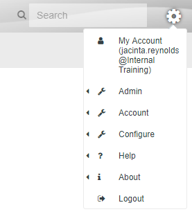
Whenever you execute a scenario(s), the status of that execution goes through to the Execution Status page.
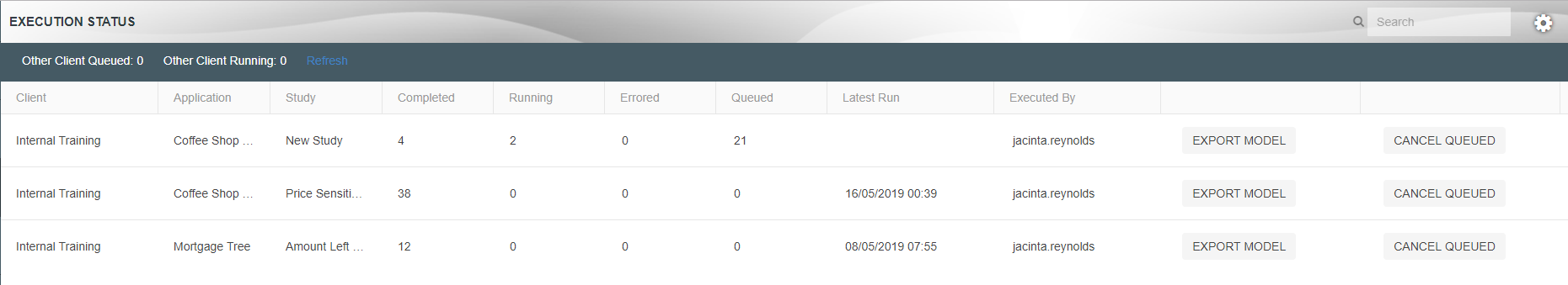
You can get ot this page in one of two ways:
 .
.In this page users can see:
The page also allows users to cancel queued scenarios and export models. If a scenario appears to be stuck running scenarios then users can come to this page and cancel the queued scenarios.
One of the features of an Akumen tenancy is the ability to export and import models in and out of Akumen. Exporting can be used to back up applications, assets, pages and datasources within Akumen, and also to transfer them between tenancies.
It is recommended that backups are created once the application is ready for use in Akumen. Whether the backup is performed through Git or through exporting, we always recommend that your models are backed up to a safe location. By default, only the Admin and Builder level roles can perform exports.
To export an application:
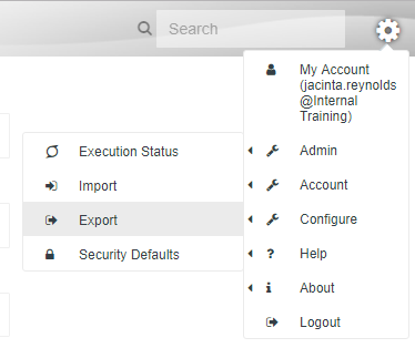
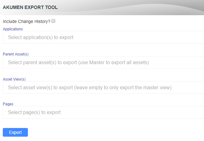
As many objects as you like can be exported, but be warned of the file size as large file downloads can result in browser timeouts. All objects exported will be in ZIP format which can be extracted if needed.
Multiple applications, assets, asset views and pages can be exported at any one time. To add add additional objects to the export list, simply click on the dropdown boxes to add them.
Pressing the hotkey Ctrl+A from within the dropdown box will select all items.
Importing is almost the same as Exporting, except that models are being brought into Akumen. Models that have been exported and now need to be reloaded in Akumen for whatever reason can be brought back using the Import page.
To import models:
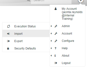
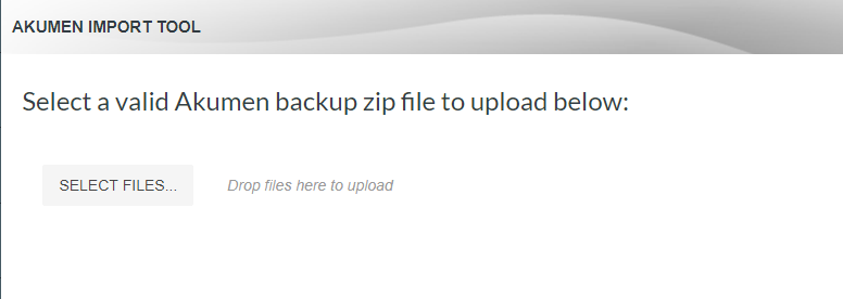
The uploaded file will need to be a zip file otherwise it will not upload correctly.
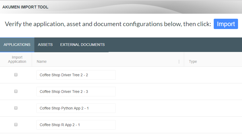
Models that already exist inside of Akumen will be numbered in the model list. For example if one copy of the model exists and you import another version the model name will appear as “Model Name - 1”. If there are two copies it will become “Model Name - 2” and so on. Note there is also an Assets tab and and External Documents tab. If there are differences between what is stored in Akumen and what is stored in Assets or Documents, these tabs provide conflict resolution.
Should anything happen in Akumen that does not appear to be a problem with the model, or you are just not sure about something that is happening, you can always check out our help options.
To get to the different help options hover over the gear symbol at the top right of the screen. From there select help. Three options will then be displayed to help you with your Akumen problem:
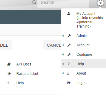
On this page we will tell you the best way to raise a ticket with our support team so that they can assist you with your issue. The API docs is covered in another section which can be found here.
Raising a ticket with our support team requires sending an email to the address of support@idoba.com. This will raise a ticket with the support team which will allow them to look into your issue and see if they can resolve the problem.
The best way to raise a ticket is to follow the following outline:
This format will provide our team with enough information to start looking into your issue/error.
Like all computer programs and platforms we recommend getting into good habits early when it comes to Akumen. This will make things like user security, version control, and maintenance of models a much easier task. The following pages are best practice suggestions and possible frameworks that we recommend for users of varying permissions and levels using Akumen.
We have covered the best practices relating to:
There are four default user roles in Akumen, and they are organized in the following way:
Use the role manager to alter these default roles and/or create new roles to suit your organisation
The following points refer to the best practices surrounding setting up security for data where different groups of users are concerned.
Users should not be an admin unless they specifically need to be. Admins can see all apps, including those that are unpublished. It is recommended that most users come under the Builder user category. This means they still do the same tasks as an admin, however they cannot see unpublished apps nor manage user accounts and security. This enables a “clean” product environment where people can work on their own creations, and then publish them for all to see once they are ready for “delivery”.
Before the roles are established, put into place an accountability system whereby only authorized people may modify the model code/driver model, and those who just need to perform scenario analysis may not. Code and driver models do not appear for those in groups that do not have model code access.
Use appropriate groups to lock down permissions at the study level. This means leaving at least one study where data is may be accessed by everyone in the appropriate groups, then lock down the more confidential studies.
Although Akumen supports setting permissions for objects for specific users, groups remain the best way to lock down permissions. This allows new people, with similar roles, to come on board and to be automatically allocated permissions without requiring someone to go through all the Akumen objects and set permissions.
Below are a list of the best practices where model versions are concerned.
For Python/R models, Akumen supports GIT integration.
For Driver Models, new versions of models need to be cloned. The model properties are such that all models have a test field for users to enter in version details for the model.
Note
Users can clone pages (including hierarchical cloning) from a completely different driver model (as long as they are authorized). This allows smaller purpose-built models to be built, and then be brought into larger models. To update the larger models, the imported pages can be deleted and reimported at a later stage.
Make use of node assumptions. Assumptions are a free text field which can have comments added to it about the node - such as where the data has come from, what the calculation solves, and what the overall model is doing.
Use Dockerfile in Py and R models to “fix” the Py and R version - Akumen can upgrade the version of Py and R in different releases.
Below are a list of best practices regarding maintaining applications, assets, and pages.
Ensure nodes are “Scoped” correctly. This means, for driver models, that the majority of the nodes have their inputs set at the application level, and a change in parameter affects all nodes in that application. Starting with v3.0, Akumen makes use of sparse input data, making large driver models extremely efficient compared to previous versions.
Utilizing the new “Copy page from another Driver Model” feature introduced in Akumen v3.0 will allow Driver Model libraries to be created. These can be small purpose built “approved” libraries that can be thoroughly tested (e.g. unit testing) using a dummy results set that can be deployed to other models using real live data.
Ensure only required inputs are sent to the research grid and results.
Make use of the Akumen Pages for those that only need scenario management, and modify inputs to give them a nicer graphical front end for entering data. They can also contain help information and data dictionaries in an easy-to-use web interface.
Ensure apps are well documented through code comments (to ensure an easy transition for new people, and an understanding for others in the organization). Driver Model calculations also support code comments, as well as assumptions, so there is no reason why apps should not be fully documented.
Ensure that all documentation of apps, permissions and users are up to date so that if and when an Administrator user has to complete a handover they can do so without causing too much confusion for the new admin. All documentation should be written as if the person reading it has no background in Akumen, this will make training and handover less stressful for all parties and allow new users to figure out how applications are built.
Need to ingest data? Datasources provide the ability to ingest both CSV and Excel files and then use the ingested data in Value Driver Models or Python and R models.
Datasources are available through the “Data” option on the left sidebar.
![]()
![]()
The “Datasource Manager” allows you to manage datasources within your Akumen tenancy. Create a new datasource by clicking on the + button in the bottom right of the “Datasource Manager” page.
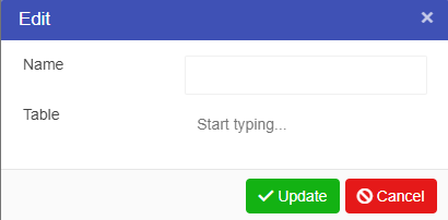
The Name specified in this window will be used to reference the datasource in other places throughout the tenancy. Once the datasource is created, it will appear in the list of available datasources.

Datasources can be edited using the right-click context menu.
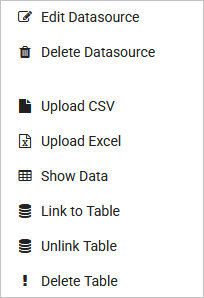
This menu allows the user to select “Edit Datasources” and edit the name of the datasource or set a model to autorun whenever an Excel or CSV upload is performed.
There is also the option to delete the datasource, but this requires the datasource to not be in use by any models.
This section outlines the common functionality between the CSV and Excel uploads.
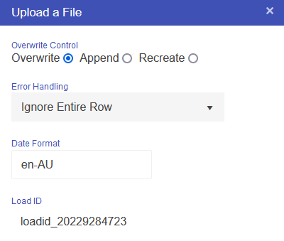
If the load id already exists in the system, all the data related to the load id will be deleted and the new data will be uploaded.
This will append the uploaded data to the existing load id.
This will drop the entire table, and recreate it in the format of the uploaded CSV/Excel file. This is useful if the format of the file has changed significantly. This will delete all data.
Error handling defines how to handle errors encounted during the load. Most errors are data type errors, eg Akumen has identified the column as a float, but the data coming through has #NA in it.
The date format specifies the expected format for loading data via CSV. As well as the date format, it is also used when converting the financial year date formats into the approriate financial year for the selected country.
Supported formats are en-AU, en-US, en-CA, fr-CA, ja-JP.
The Load Id is an important concept in datasources. It provides the ability to reference individual data “loads”. The Load Id can be autogenerated or user entered. Querying datasources through Python or VDM can reference the load id to only fetch a subset of the data within the database.
The load id selection is an autocomplete box that detects other load ids to assist in selecting an existing one for overwrite.
Incoming data can be in either Long format:
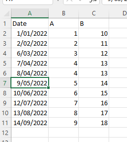
Or Wide format:
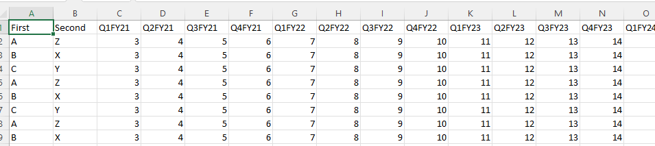
If data is in wide format and Akumen detects dates in the headers, it will convert the dataset to long format for ingestion. All of the “category” columns are retained, but a new column is created called “date” where the date values are copied into, and a new column called “value” is created, where all the values are copied into. Basically a new row is created for every cell within the wide format data.
In addition, dates can either be valid dates, or as in the example above, financial year references. Supported formats are Q1FY22, H1FY22 or FY22, and convert it to the appropriate financial year timestamp for storage. See above for valid date formats.
Once the upload has successfully completed, the configuration (with the exception of the load id) will be saved for the next upload on the same datasource.
When using datasources in a Value Driver Model, at least one column must be able to be converted into a date/time, and at least one column must be able to be converted into a valid number.
This section outlines the functionality required to upload a CSV.
There are no additional settings required for a CSV outside the common settings.
This section outlines the functionality required to upload an Excel Spreadsheet.
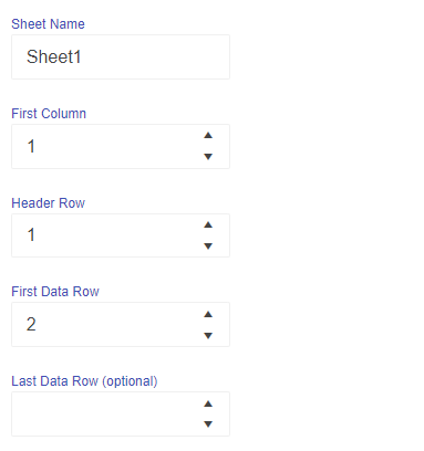
The settings for an Excel spreadsheet upload are 1-based, which means the uploaded data structure starts at 1 instead of 0.
The settings for uploading an Excel spreadsheet are:
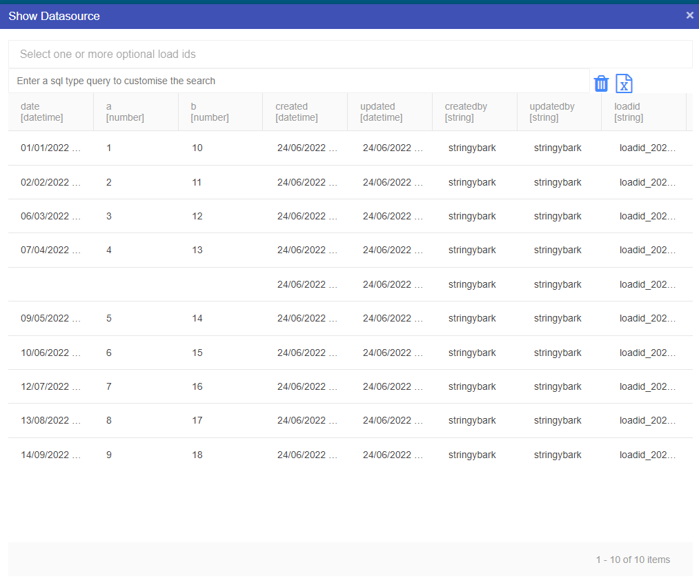
Clicking on the Show Data right click menu option opens the Show Data window. By default, it shows a tabular view of all data.
At the top of the screen, one or more load ids can be selected to filter the data.
Under the load id, a user entered sql based query can be entered. In the example above, something like a < 4 will filter the data to only show rows where “a” is less than “4”.
The delete button behaves in two ways:
The Excel button exports the dataset to Excel, honouring the load id and filter that is applied.
The right-click context menu contains separate options for linking and unlinking tables.
When linking a table to a datasource, the user can select any table already existing in the tenancy. The data in this table will then be available to any model referencing the datasource. The same table can also be linked to multiple datasources.
Unlinking a datasource simply removes its connection to the underlying table. The datasource will still exist and can be be linked to the same table or other tables.
A “Datasource” node type exists in Value Driver Models which is used to reference datasource data within the model. For more information on using datasource nodes in Driver Models, see here.
Python applications have similar functionality but instead use a “datasource” variable type. Further information on this can be found here.
Applications can support one or more load ids. There is also the option to specify an additional query to limit datasource data.
It is possible to delete underlying datasource tables from the “Datasource Manager” by selecting the “Delete Table” context menu option after right-clicking an existing datasource record.
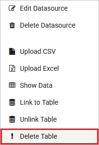
There must be no models referencing a datasource table before it can be deleted. If there are models referencing it, the names of these models will be provided in the error message when the deletion attempt is made. If this occurs, the user simply has to remove the datasource node references within the model. Alternatively, the model can also be deleted if it is no longer required.
Model deletions are permanent and cannot be undone. This also applies to the deletion of datasource tables.
In this tutorial we will step you through the Akumen workflow by modelling a basic coffee shop.
John would like to invest $10,000 and open his own coffee shop. John’s good friend Jack will contribute his coffee machine to the start-up. However, Jack does not like risks and therefore wants to be employed by John rather than partnering. They have already found the location, but they believe they need 10 weeks to set it up as a café. John is wondering when he will make a return on his investment and Jack wants to know what the price for a cup of coffee should be.
First, we will create a driver model to calculate the business’ cash reserve and when John will break even, then we will explore scenarios around the best price for a cup of coffee (their only product).
With this is a simple example we will show you how to use Akumen and its capability to explore situational scenarios based on “What-if…?” questions.
We will model our Coffee Shop in increments.
The Asset Library is one of the most important parts of Akumen. It stores fixed pieces of information for models to draw on. Before we can start building our coffee shop model we need the fixed data surrounding this coffee shop. Data such as monthly rent and how much it costs to produce a cup of coffee are fixed pieces of information the needs to be kept consistent in order ot produce accurate results.
To do this we will use the Asset Library. In the asset library we can store this information only updating the values when necessary. For more information on how to use the Asset Library and the different things you can do with Assets in the Asset Library click here.
In the Asset Library you will notice that on the left hand side of the screen is a list of all the current Asset Templates and in the middle is the Master Asset which houses all of the Assets currently sitting in the Asset Library.
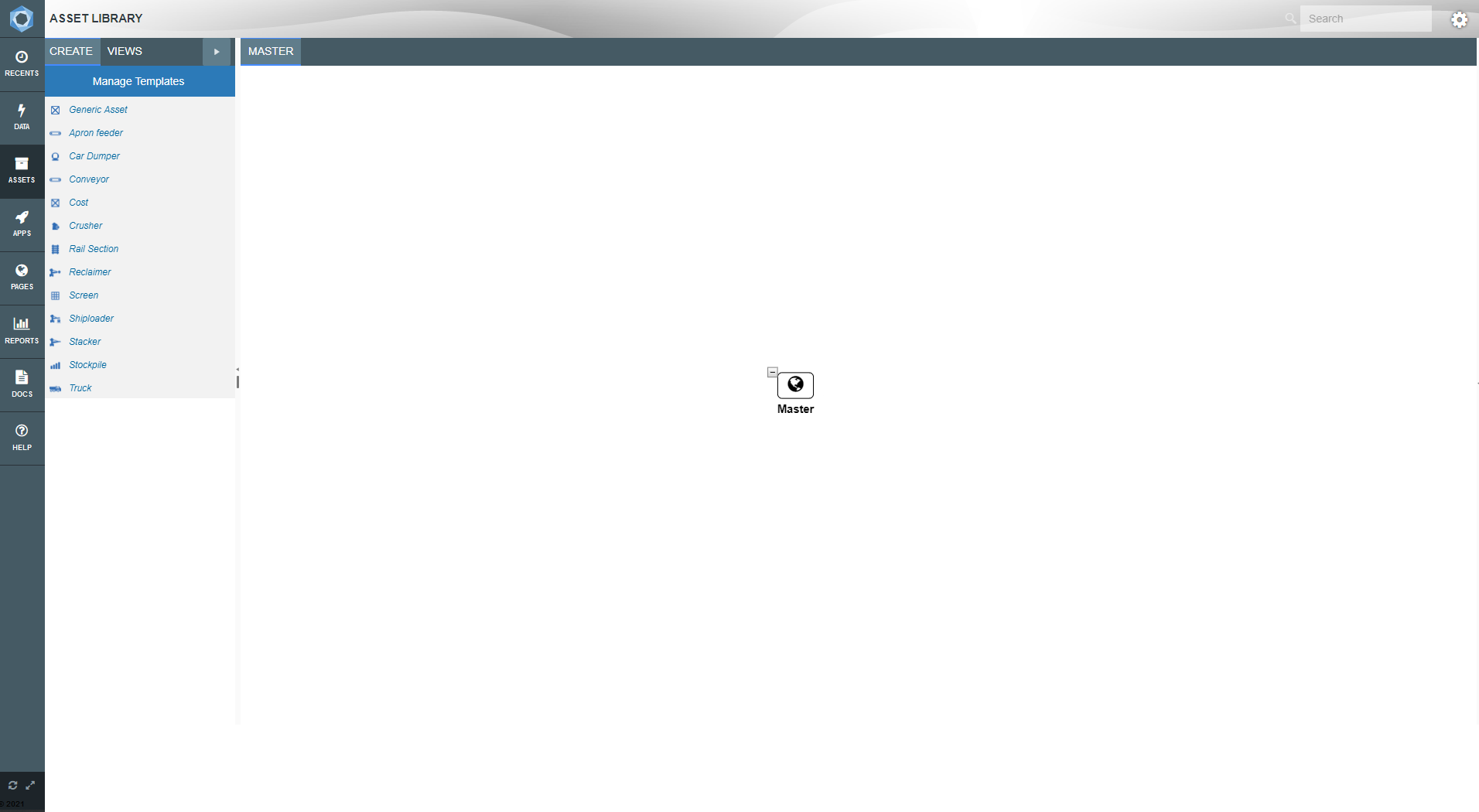
It is always best practice when creating a new branch in the Asset Tree to create Asset templates for Assets that do not currently have an Asset in the template list. We do not have a template for a Coffee House, or a Coffee Machine in Akumen therefore we need to create two new templates for these two assets.
We need to add one attribute to both the Coffee House and the Coffee Machine.
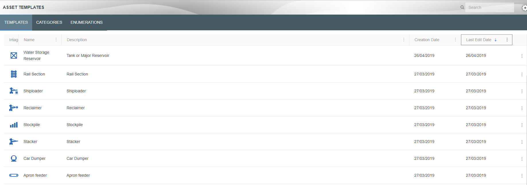
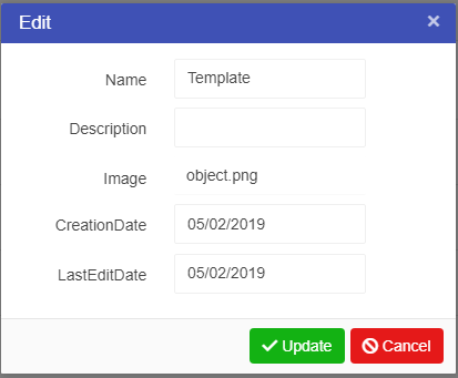
Now that we have our two Asset templates we can add some attributes to them. Attributes allow users to to store values in Assets (for more information on Asset Attributes click here).
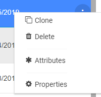
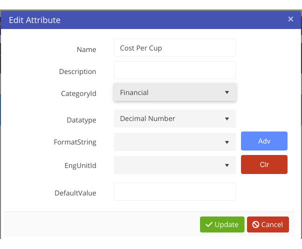
Our templates are ready to use in setting up the Asset Library
We now have our new Assets Templates for the coffee shop and Attributes defined that will let us store relevant data in the Asset Library. We can now create assets from the templates and fill in the attribute values against the appropriate assets.
For this tutorial we be creating three Assets:
All three are different templates, two of which we have already built the other is a pre-made Generic Asset.
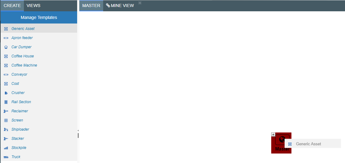
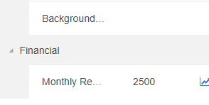
We have now put all our Asset information into the Asset Library
Please click here for instructions on how to create and configure Driver Model Applications
To create an Application for our Driver Model:

Akumen will take you directly to the Driver Model Workspace
We will be building the model of John’s Coffee Shop incrementally. First, we will be modelling its operational income and then we will be adding in the fixed overhead costs. Last, we will address the shop’s cash reserve at the bank.
Before we start, we need to delete the demonstration nodes that are created by Akumen when a Value Driver Model is created. Click and hold on an area of the canvas, and drag the mouse so all the nodes are covered by the square. Release the mouse, and all nodes will be selected. Hit the delete key and accept the prompt to delete all of the nodes.
Our Driver model will be modelled in three parts:
Because of this we will need three Driver Model Pages. On the left hand side of the screen you will see the pages window. We will create two sub pages from the page titled Initial Page so that we can create the different parts of the Driver Model.
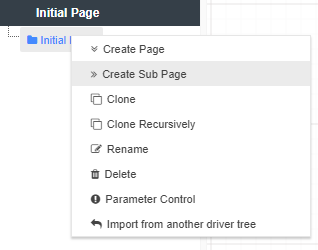
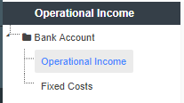
Now go to the Operational Income page. On this page we will start building our Driver Model based on the operational income.
Jack knows from experience that one cup of coffee from his Italian coffee machine costs $0.5. This is the value he would like every app to use. Hence, we put it into the Asset Library.
The Asset Node on the Driver Model has a permanent link to the Asset Library. If the value of the property in the Asset Library changes, the new value will propagate to all the applications that use that property. Akumen will also create an audit trail for this property which allows users to confirm from where the value came thus giving you full traceability of, and control over the crucial numbers in your business.
You will notice the different colours indicate different nodes. For example, a Numeric Node is green, an Asset Parameter Node is blue. For more information on the different types of nodes click here.
 to bring up the properties bar on the right side of the screen.
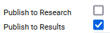
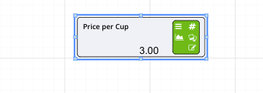
The Publish to Results tick box must be ticked in all nodes that you wish to see the results for, otherwise the values for that node will not appear in the Data tab. The nodes that are published to results have a small chart icon, and publish to research have a “hamburger” above the publish to results icon.
Now that we have our two starting values we can add our Calculation node to work out how much money would be made per cup of coffee sold.
[Price per Cup]-[Coffee Machine.Cost Per Cup].Now that we can calculate the profit per cup we need to get to our operational income, and to get that we need to add in an estimation of our monthly sales – the quantity of cups poured.
From market research, John knows that the demand for coffee in his area is a function of price. He has determined that the quantity of cups demanded per month is equal to approximately 3500 – 100 * [Price per Cup] ^ 2. However, this function does not describe his observation fully. The demand for coffee also seems to be affected by a random “noise” that John cannot explain. He decides that this noise should be modelled by a standard distribution with a mean of 0 and a standard deviation of 150.
The first thing we will do is add a Distribution node to the Driver Model. After that we will calculate the demand per month.
on the Distribution node.3500 – 100 * [Price per Cup]^2 + [Demand Noise].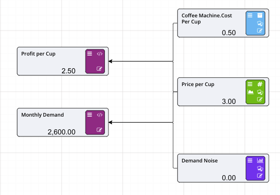
Before we can forecast the operational income of the coffee shop, we need to account for another detail in our case study. Remember:
John and Jack believe they’ll need 10 weeks to set-up their new shop in the leased property.
In other words, it will take 10 weeks before they may sell their first coffee and start satisfying the demand that we calculated in the previous section using the Distribution node. For that reason, we are going to add in a Timeseries node that models the months in operation (for more information on Timeseries nodes click here).
The editor supports excel-like dragging of values across cell. Select the little blue circle of the cell marker for this purpose.
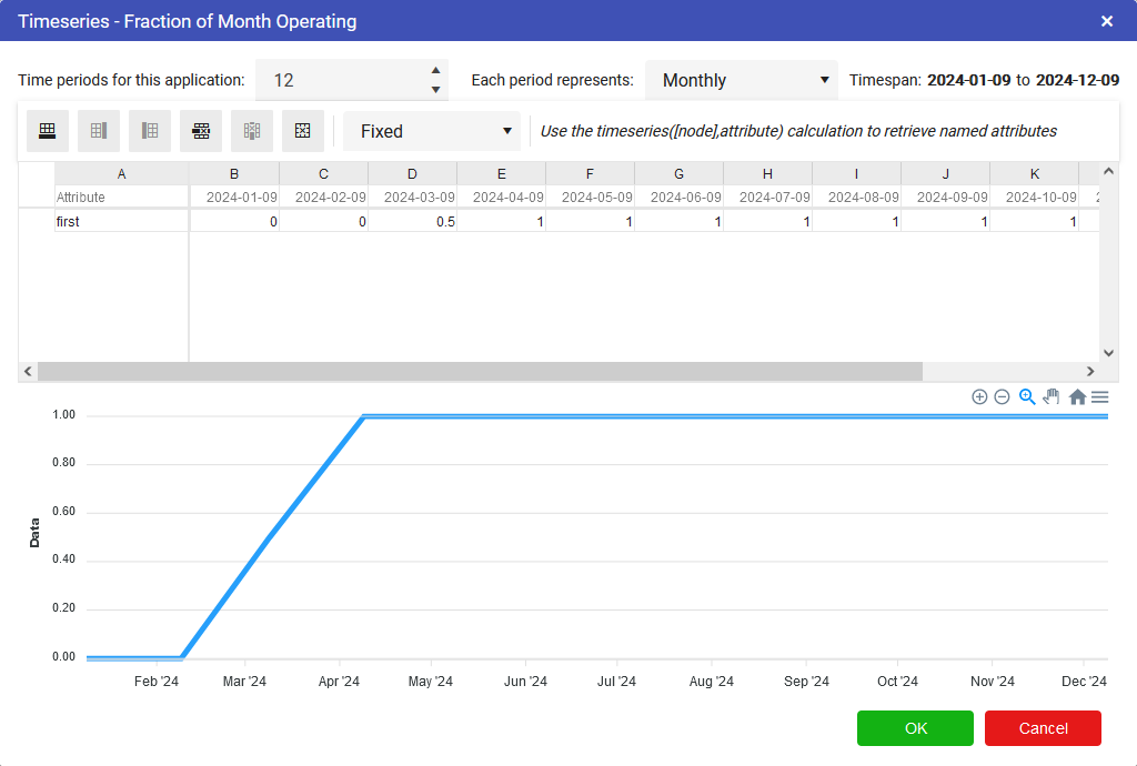
We now have our Timeseries node now, so we can now work out the monthly income while the Coffee Shop is in Operation.
Add a new Calculation node to the left of your previous calculations and rename it to Monthly Income.
You can use the mouse to click and drag to pan around the driver model, or the scroll wheel of your mouse to zoom in and out if you start to run out of space on this page.
Info
Connect the timeseries and the other two calculations (Profit per Cup and Monthly Demand) to the new Calculation node.
Set the expression for the new calculation to: [Fraction of Month Operating] * [Monthly Demand] * [Profit per Cup].
Confirm the driver model looks like.
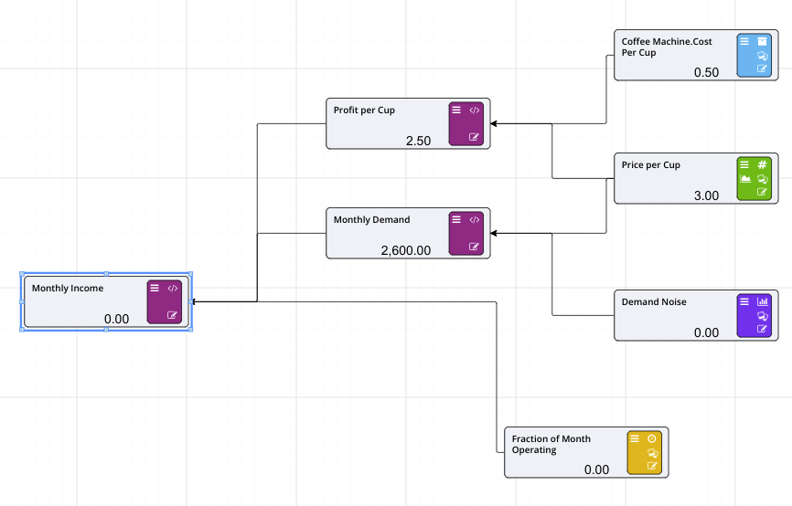
We now have a forecast of the operational income for John’s coffee shop. Now that we have this we can go and model the fixed overhead costs.
The fixed overhead costs are the next part of this coffee shop Driver Model. For this part of the tutorial we will use calculation nodes to calculate the total fixed overhead costs. To start this part of the Driver Model go to your Driver Model page titled Fixed Costs. We have a little bit of information regarding some of the fixed costs for this coffee shop. The first is the monthly rent we put into the Asset Library as part of the Coffee House Asset. The second is that Jack, who is lending the coffee machine, wants to be employed rather than a partner. Jack says that his salary will likely be 2400 a month.
First we will set up the inputs:
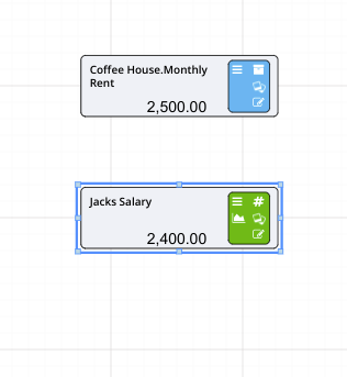
Now that we have our primary inputs, we can start adding them together using a calculation node.
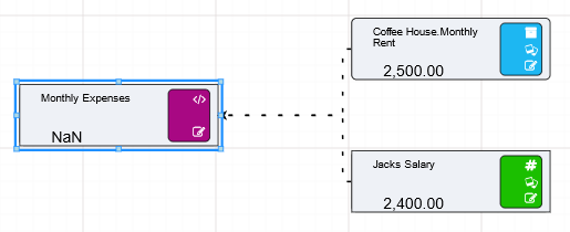
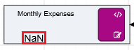
[Coffee House.Monthly Rent] + [Jacks Salary] in the expression editor.
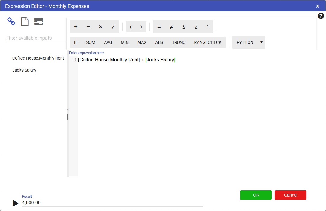
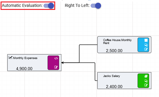
Getting the results of the two separate Driver Models onto one page requires the use of the Node Reference node. This node will take any value from any Driver Model on any of the other Driver Model pages and bring them into the current page. We will use Node Reference nodes to connect the two separate Driver Models we have just created and use them in the final one to work out the cash reserves at the bank according to the modelled income and expenses. For more information on Node Reference nodes click here.
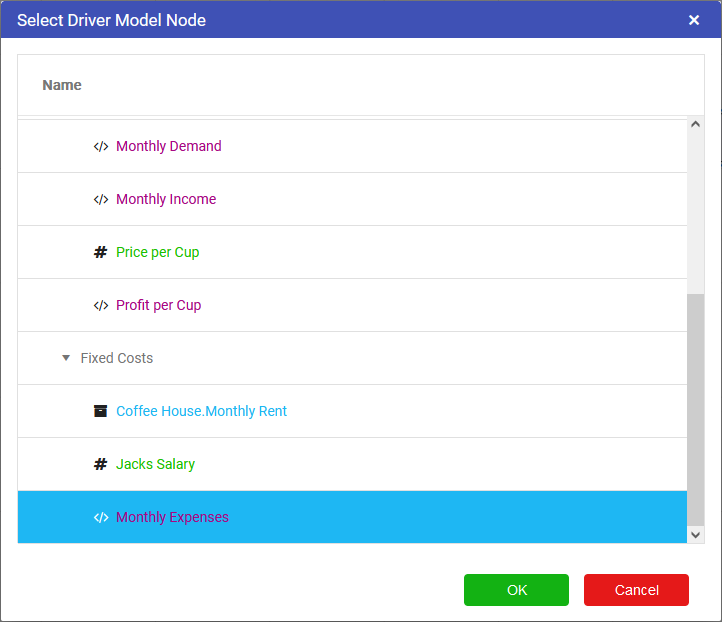
[Monthly Income]-[Monthly Expenses].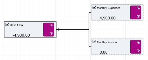
Now that we have connected our two driver models together we need to work out what the end of month balances will be for the shop so we can find out when John will make start making a return on the Coffee Shop.
To complete the model we need to add one more node, the Prior Value node. The Prior Value node will allow us to sum up the end of month balances to find out when there will be a return on the $10000 originally put into the coffee shop.
Prior Value Nodes are used to access the value of a node from the previous time step. They are especially useful for calculating balances. Driver Models typically calculate the closing balance and the Prior Node is used to determine the opening balance, today’s opening balance is yesterday’s closing balance (for more information on Prior Value nodes click here).
Prior Value Nodes are different to normal nodes in that they have two separate input ports; one on the left and one on the top. The top port is for the initial or starting value of the node and provides a value from before the first timestep, ie t = -1. This value will be used for the first timestep in the series. When the initial value is zero this input port can be left empty. The second port is for the closing value that will become the starting value for the next timestep. Hovering over each port will display a tool tip with information on the purpose of each port.
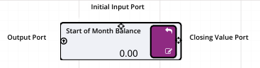
[Start of Month Balance]+[Cash Flow] by dragging the two connected assets from the list into the editor.Your Driver Model should look like the image below.
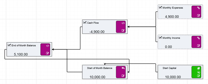
Ensure the Automatic Evaluation toggle is on, then step through time to see when John will make a return on his coffee shop. You should find that by the tenth timestep the End of Month Balance should be 11350, so we can say that John will make a return at around 11 months.
Before moving on to the Research part of this tutorial make sure that you have ticked the Publish to Results tick box in the properties bars of the nodes in your Driver Model. A quick way to set all nodes to Publish to Results and Publish to Research is to right click on a page (eg the Bank Account page), and select the Parameter Control option. This enables the toggles for all nodes on the page. Click Recurse Child Page to set it for all pages.
You have now completed a Driver Model. The next part of the tutorial is using the Research Grid to find the best price for a cup of coffee to maximize the return. Proceed to research to learn how to research the coffee shop findings, or click here to build the same application in Python or here to build the same application in R
There are three ways to model John’s Coffee Shop. In this part of the tutorial we will take you through how to model the coffee shop using Python code.
To create a Python application:
Akumen will take you directly to the code editor screen
We will be building the model of John’s Coffee Shop incrementally. First, we will be modelling its operational income and then we will be adding in the fixed overhead costs. Last, we will address the shop’s cash reserve at the bank.
To know more about creating Python and R applications and how to configure them click here
When you create a new application in either Python or R Akumen will take you to the code editor screen.
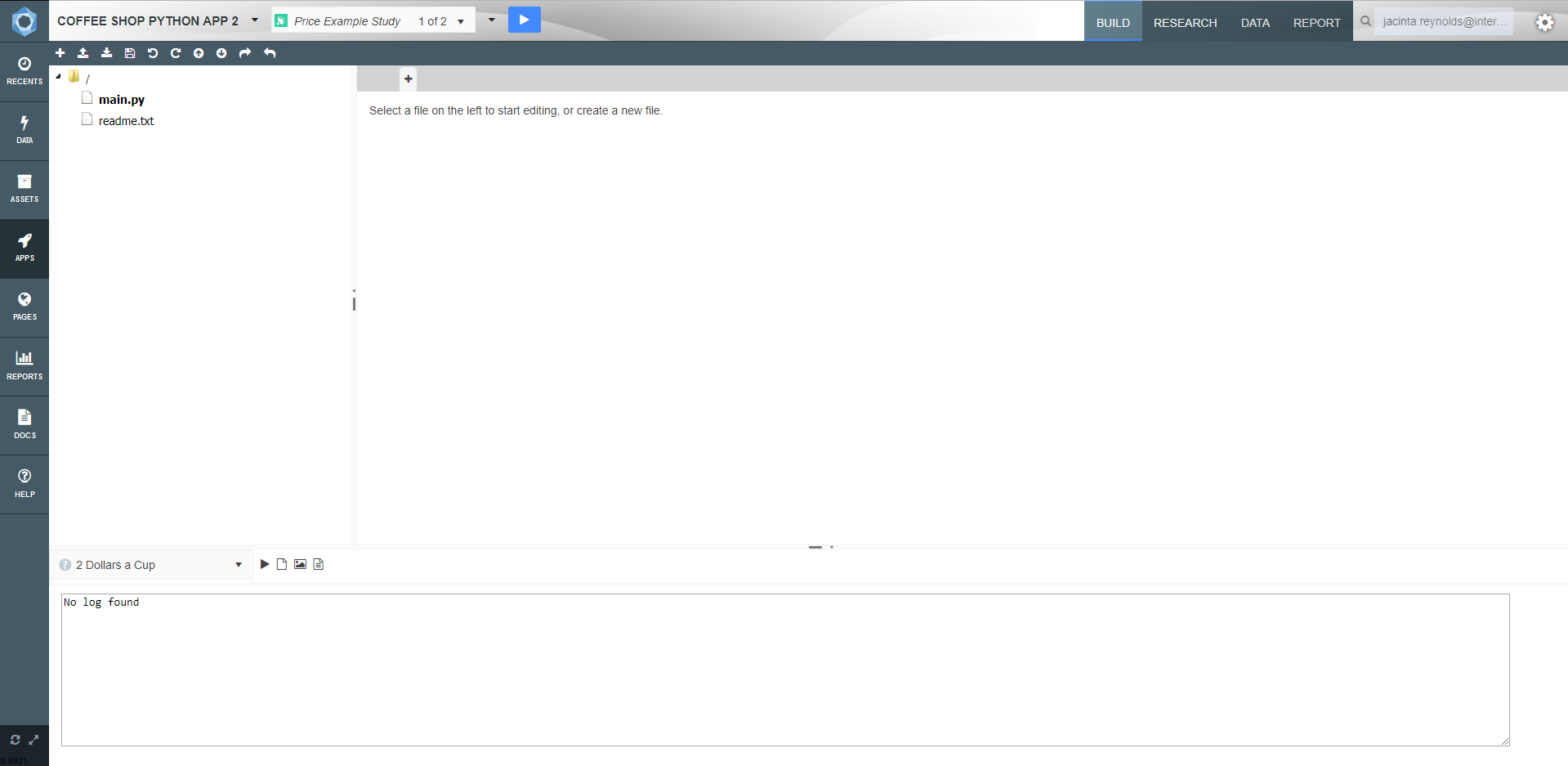 There are Five main areas to the Code editor screen:
When Akumen first creates a Py model, it automatically creates an initial main.py file.
To create a new file:
The above will start our model off by allowing us to set a start date and enter the amount of time periods we will be using in the model.
Assigning a parameter to the Application Level Parameters applies the assigned value to all scenarios across the entire application. Assigning a value to the Study Level Parameters applies the assigned value to all scenarios within a single study. Any value in either of these cells will not be displayed in the scenarios within the studies.
In order for Akumen to execute your Python code, we need to define an akumen(…) Python function. This function is the main entry point for your code and must exist in the execution file. The Akumen function must either take keyword arguments (**kwargs) or parameters matching Akumen parameters as input.
The readme file contains handy hints on information on syntax for creating the main.py file. This includes how to define variables that are used in the research grid
John would like to invest $10,000 and open his own coffee shop. John’s good friend Jack will contribute his coffee machine to the start-up. However, Jack does not like risks and therefore wants to be employed by John rather than partnering. They have already found the location, but they believe they need 10 weeks to set it up as a café.
From market research, John knows that the demand for coffee in his area is a function of price. He has determined that the quantity of cups demanded per month equals approximately to 3500 – 100 * [Price per Cup]^2. However, this function does not describe his observation fully. The demand for coffee also seems to be affected by a random “noise” that John cannot explain. He decides to model this noise through a standard distribution with a mean of 0 and a standard deviation of 50.
John is wondering when he will make a return on his investment and Jack wants to know what the price for a cup of coffee should be.
To start modelling John’s coffee shop we need to first define what parameters contribute to the operational income. These parameters are:
We then need to work out what the costs to the cafe are. Currently they are the shop rent and Jack’s salary. We also know that we have a start capital of $10000. Most of these will be float values in Python, two will be asset values, and a few of our parameters will be put into a tabular entry.
Switch back to the Build tab, open the main.py file, and overwrite the contents of the file with the following code
We have a number of float values in our Python code. Float values can be assigned as Assets or can be entered as numbers or dates by users. These are the values we are going to enter first. After the float values we will address adding assets and editing tabulars to finish modelling the operational income of the coffee shop.
First we will look at entering in our float values:
Linking Assets into Python code can be done in two ways:
For this tutorial we will attach our two assets to the Python code as values through the Research Grid. We know that two of our values, cost per cup and monthly rent, are already in the Asset Library (if this is not the case go back to the Asset Library page and Asset Library Template page to create your Assets)
To attach the Assets to the Python code as values:
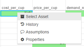
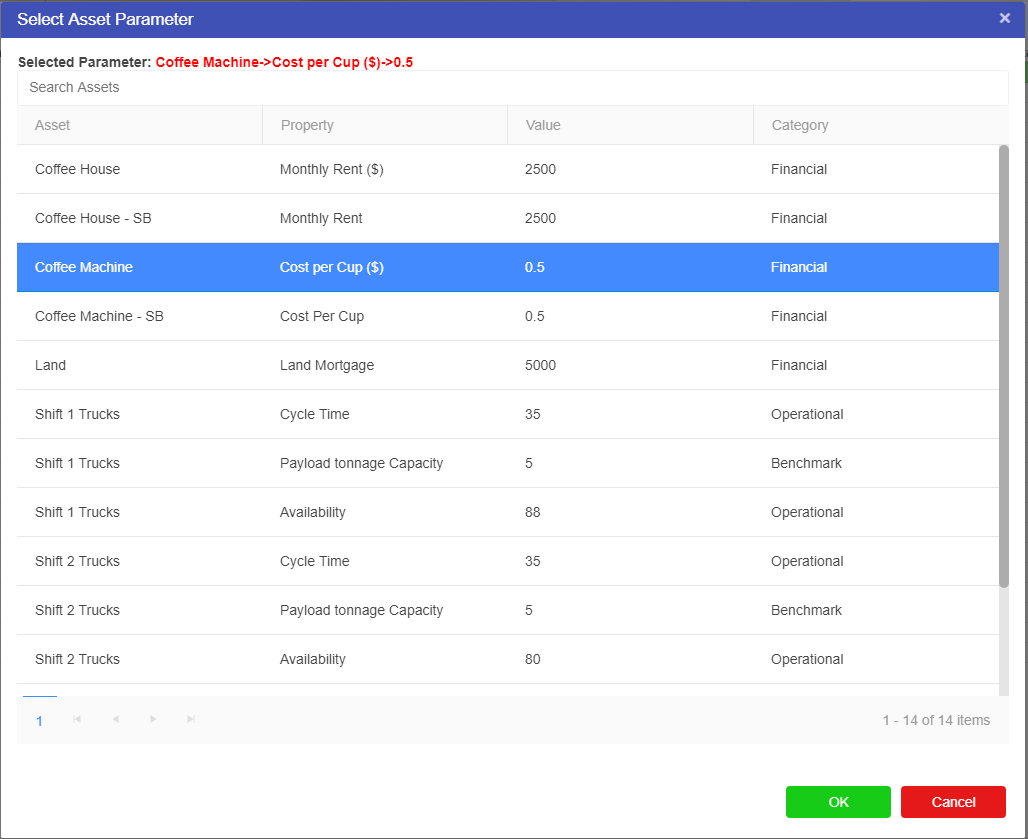
We have now entered our float values and attached our Assets, the last step we have is to enter data into our tabular input. This tabular will allow us to work out what fraction of the coffee shop will be operational over the course of the 12 months we are modelling. John and Jack believe that it will take 10 weeks before their coffee shop is ready to sell coffee. This means that for the first two months and half of the third month of the year they will not be able to sell any coffee at their cafe.
The tabular will reflect the operational months, and since this fraction will not change from study to study we can set up this table in the Application Parameters Level row. To set up the tabular:
This spreadsheet is very similar to an Excel spreadsheet and supports the same basic features as an Excel spreadsheet. It can upload excel spreadsheets and when data is downloaded from the cell it will display as an excel .csv.
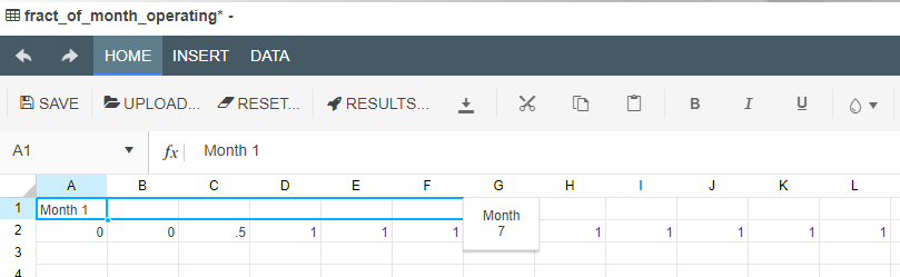
You can use the same click and drag feature for months for the other cells all requiring a fraction of 1 in them.
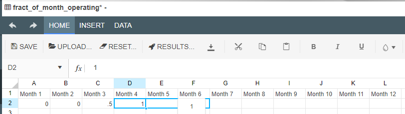
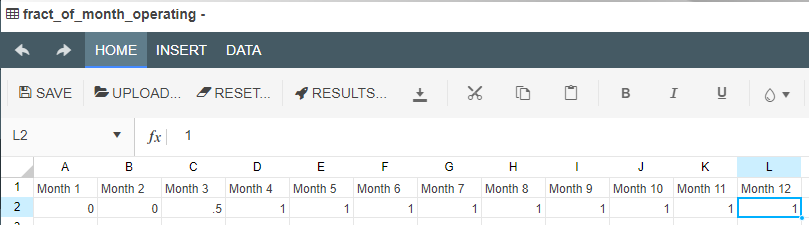
Now that we have set up our tabular data we can say that we have finished modelling our operational income. The next step requires putting a few more lines of code in to model the fixed costs and produce the final bank account values at the end of the month.
Now that we have modelled our operational income and filled in all the relevant values into our Research Grid we can model our fixed costs and set up the code to find the final bank balance at the end of every time step which for this model is at the end of every month.
To model the Fixed costs and find the final bank balance we will need to exit the Research Grid and go back to the Build screen and our code editor.
Once in the build screen put the following lines of code at the top of the model:
These lines of code will allow the model import the necessary libraries to complete the calculations needed in our next few lines of code and allow us to model the noise demand that we have already defined as part of our operational income.
Once these lines are in replace the return {} at the bottom of the model with the following code:
The above lines of code not only Calculate the income and the costs, but also model the distribution noise, create timesteps in the model and work out and write the final bank balances to the Results tab. This is now a workable model of John and Jack’s coffee shop.
You have now completed a Python Application in Akumen. The next part of the tutorial is using the Research Grid to find the best price for a cup of coffee to maximize the return. Proceed to research to learn how to research the coffee shop findings, or click here to build the application in a Driver Model or here to build the application in R code.
Akumen can return charts, plotted through Python libraries such as MatPlotLib. By adding the following code to your Python coffee shop application you will be able to view the results of the model once the scenarios have been run. Add the following code to the bottom of the Python application, just before the return{}.
Once you have added the code and saved your changes, rerun your model to produce new data. As soon as the scenarios have run and returned complete you can view the charts in a few different ways:
The completed main.py file should appear as follows:
There are three ways to model John’s Coffee Shop. In this part of the tutorial we will take you through how to model the coffee shop using R code.
To create a R application:
Akumen will take you directly to the code editor screen
We will be building the model of John’s Coffee Shop incrementally. First, we will be modelling its operational income and then we will be adding in the fixed overhead costs. Last, we will address the shop’s cash reserve at the bank.
To know more about creating Python and R applications and how to configure them click here
When you create a new application in either Python or R Akumen will take you to the code editor screen.
There are Five main areas to the Code editor screen:
When Akumen first creates a Py model, it automatically creates an initial main.py file.
The above will start our model off by allowing us to set a start date and enter the amount of time periods we will be using in the model.
Assigning a parameter to the Application Level Parameters applies the assigned value to all scenarios across the entire application. Assigning a value to the Study Level Parameters applies the assigned value to all scenarios within a single study. Any value in either of these cells will not be displayed in the scenarios within the studies.
In order for Akumen to execute your R code, we will need to specify the main entry point for Akumen, which means we will need to define an ‘akumen’ function. This function is the main entry point for your code and must exist in the execution file. The akumen function will require the form: akumen <- function(first, second, ...) {}
The readme file contains handy hints on information on syntax for creating the main.r file. This includes how to define variables that are used in the research grid
John would like to invest $10,000 and open his own coffee shop. John’s good friend Jack will contribute his coffee machine to the start-up. However, Jack does not like risks and therefore wants to be employed by John rather than partnering. They have already found the location, but they believe they need 10 weeks to set it up as a café.
From market research, John knows that the demand for coffee in his area is a function of price. He has determined that the quantity of cups demanded per month equals approximately to 3500 – 100 * [Price per Cup]^2. However, this function does not describe his observation fully. The demand for coffee also seems to be affected by a random “noise” that John cannot explain. He decides to model this noise through a standard distribution with a mean of 0 and a standard deviation of 50.
John is wondering when he will make a return on his investment and Jack wants to know what the price for a cup of coffee should be.
To start modelling John’s coffee shop we need to first define what parameters contribute to the operational income. These parameters are:
We then need to work out what the costs to the cafe are. Currently they are the shop rent and Jack’s salary. We also know that we have a start capital of $10000. Most of these will be float values in R, a two will be asset values, and a few of our parameters will be put into a tabular entry.
Switch back to the Build tab, open the main.r file, and overwrite the contents of the file with the following code
We have a number of float values in our R code. Float values can be assigned as Assets or can be entered as numbers or dates by users. These are the values we are going to enter first. After the float values we will address adding assets and editing tabulars to finish modelling the operational income of the coffee shop.
First we will look at entering in our float values:
Linking Assets into R code can be done in two ways:
For this tutorial we will attach our two assets to the R code as values through the Research Grid. We know that two of our values, cost per cup and monthly rent, are already in the Asset Library (if this is not the case go back to the Asset Library page and Asset Library Template page to create your Assets)
To attach the Assets to the R code as values:
We have now entered our float values and attached our Assets, the last step we have is to enter data into our tabular input. This tabular will allow us to work out what fraction of the coffee shop will be operational over the course of the 12 months we are modelling. John and Jack believe that it will take 10 weeks before their coffee shop is ready to sell coffee. This means that for the first two months and half of the third month of the year they will not be able to sell any coffee at their cafe.
The tabular will reflect the operational months, and since this fraction will not change from study to study we can set up this table in the Application Parameters Level row. To set up the tabular:
This spreadsheet is very similar to an Excel spreadsheet and supports the same basic features as an Excel spreadsheet. It can upload excel spreadsheets and when data is downloaded from the cell it will display as an excel .csv.
You can use the same click and drag feature for months for the other cells all requiring a fraction of 1 in them.
Now that we have set up our tabular data we can say that we have finished modelling our operational income. The next step requires putting a few more lines of code in to model the fixed costs and produce the final bank account values at the end of the month.
Now that we have modelled our operational income and filled in all the relevant values into our Research Grid we can model our fixed costs and set up the code to find the final bank balance at the end of every time step which for this model is at the end of every month.
To model the Fixed costs and find the final bank balance we will need to exit the Research Grid and go back to the Build screen and our code editor.
Once there, copy the code below over the “return ()” statement at the bottom of the main.r file, ensuring that the closing bracket has not been copied over:
The above lines of code not only Calculate the income and the costs, but also model the distribution noise, create timesteps in the model and work out and write the final bank balances to the Results tab. This is now a workable model of John and Jack’s coffee shop which we can use for finding answers to their two questions:
The completed main.r file should appear as follows:
Akumen’s R integration supports most functionality of R and there are no differences in syntax or semantic.
You have now completed an R Application in Akumen. The next part of the tutorial is using the Research Grid to find the best price for a cup of coffee to maximize the return. Proceed to research to learn how to research the coffee shop findings, or click here to build the application in a Driver Model or here to build the application in Python.
In one or more of the previous sections, you will have built your coffee shop model. This simple model can be executed to generate a set of results for users based on the scenario inputs. However, two of Akumen’s key-capabilities are its scenario generation and scenario management functionalities.
Scenarios allow users to determine the applications response to different inputs.
For example, we can ask: “If the price of my product is X and the number of sales Y is a function of the price, how much Revenue will I earn?” Here, X is an input, Y is a calculation and Revenue is a calculated output.
Now, we can ask “What-If?” questions by changing our inputs and seeing what the output will be. This is called a Scenario.
“Scenario 1: What if I priced my product at $2?”
“Scenario 2: What if I priced my product at $4?”
“Scenario 3: What if I priced my product at $5?”
Akumen allows you to create hundreds of scenarios to determine configurations that deliver the best outcome. In this research process, you may want to change parts of your model as you get more insights into your model’s behavior. Akumen manages those changes for you to ensure your model stays consistent across scenarios in areas where it should and differs where it matters. This is achieved through the Scope property of a parameter.
Please click here for further instructions on how to use the Research tab, grid, cloning and flexing scenarios.
Users can group scenarios into a study. A study is a collection of scenarios that aim to answer a particular question. In our case we will be studying price sensitivity.

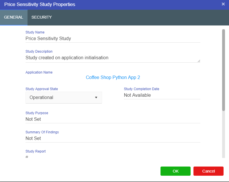
Now that we have renamed our study to describe what we are going to do we can start creating scenarios to find the best price for a cup of coffee for John and Jack.
To proceed further in the tutorial one of the Coffee Shop App types (Driver Model, Python or R) must already exist. All of the following steps in the tutorial can be applied to any of the Coffee Shop App types.
Cloning scenarios allows us to create an exact copy of another scenario. This allows us to change a value between scenarios to see how this value affects the results of the new scenario from the original, or baseline scenario (for more information about cloning scenarios click here).
We want to start off by cloning our baseline scenario. To clone or flex and answer our “what-if” questions surrounding our coffee shop we must be in the Research Grid of our coffee shop application.
Once inside of your coffee shop application you will want to go to the Research Grid which can be found by clicking on the Research tab at the top right of the screen.
 Once you are in the Research Grid you will see the baseline scenario at the very top of the grid. This is always the best scenario to clone for any new scenario. The first scenario created by default becomes the baseline scenario, but once there are more scenarios in a study a new baseline scenario can be chosen by users. The baseline scenario is the scenario carried into new studies when they are created by users.
Now that we are in the Research Grid it is time to clone a new scenario. The new scenario we will create looks at “What if $2 dollars was charged for a cup of coffee?”. To clone a scenario and answer our “what-if” question:
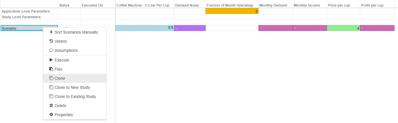
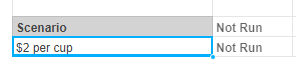
Now that we have cloned a scenario we can change the value of the price per cup and compare the results of the new scenario against the baseline. To set up this scenario:
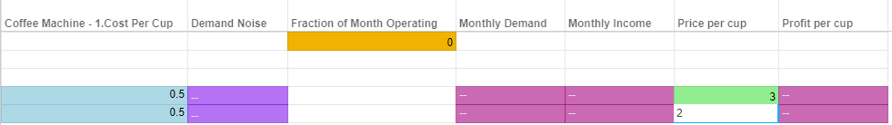
To view the results of the two scenarios you will need to execute the scenarios. To execute the scenarios either:
For more on executing scenarios click here
If you are researching the VDM tutorial, you will notice the timeslider is still at the bottom of the screen. This allows you to step through time in the same way as in the build screen.
We have now cloned our scenario and have the results of charging customers paying $2 for a cup of coffee. Now we will flex our baseline scenario so we can analyse lots of results all at once without having to clone all of the scenarios individually.
Akumen provides you with the ability to generate input values across a user specified range. This is called flexing (for more information click here). With flexing you are able to generate hundreds of different scenarios across a specified range. This is particularly useful for our current tutorial where we are trying to find out what the best price is for a cup of coffee.
Since John and Jack want to find the best price for a cup of coffee we must look at lots of different prices over a certain range. It is suspected that the best price is somewhere between $2.5 and $5. When flexing in any study in any application it recommended that users flex the baseline scenario.
To flex our baseline scenario:
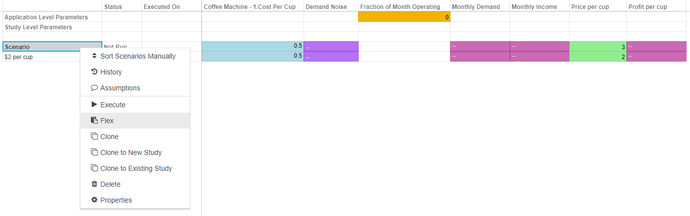
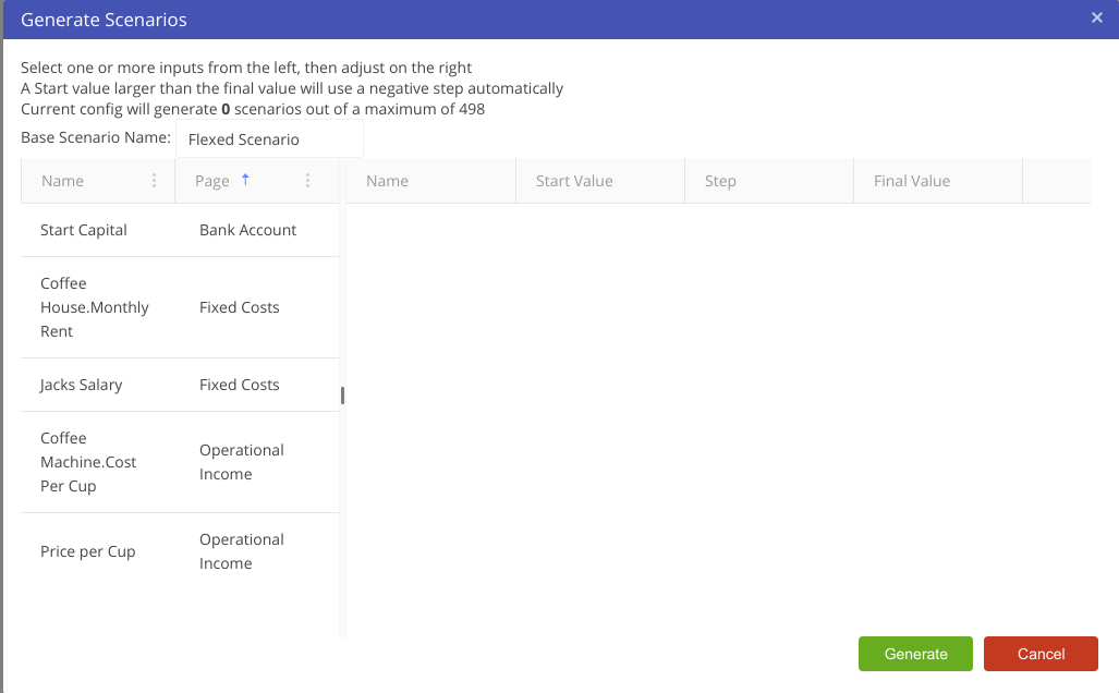
Price per cup variable.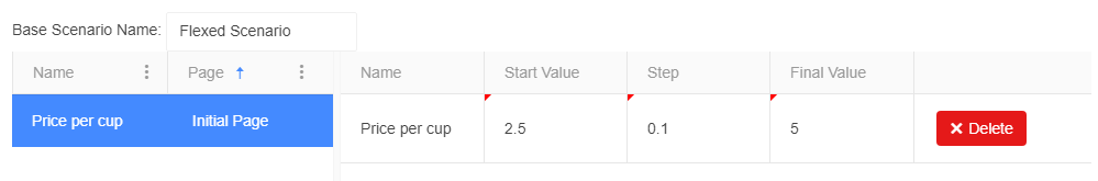
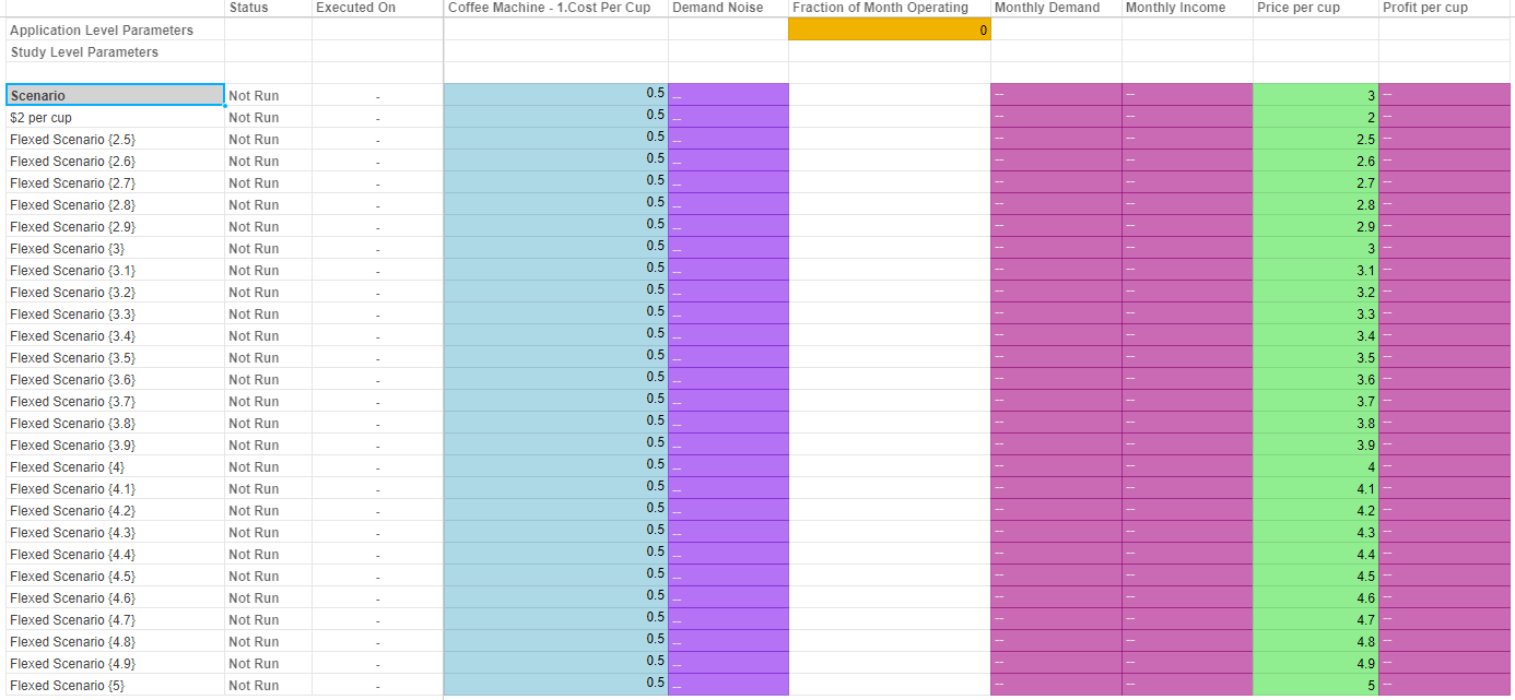
Once generated, the created scenarios are ready to be executed so that we can use the results to find the best price for a cup of coffee. To execute all the scenarios click the blue play button at the top of the page, this will allow you to execute all scenarios in the current study.
We will be able to analyse these results and find the best price for a cup of coffee by looking at the Results in the Reports section of the tutorial. But first we show you how to view and, if needed, download your raw data.
If you go to the Data tab at the top right of the page (next to the Research tab) you will find the raw results of the scenarios that have executed and have run without error and returned complete. Scenarios that have run but returned an error will not display any results in the Data tab.
The data tab provides a user the ability to view and query the raw data that is generated by applications. This functionality works in the same way regardless of the language (Driver Models, Python or R) that is used.
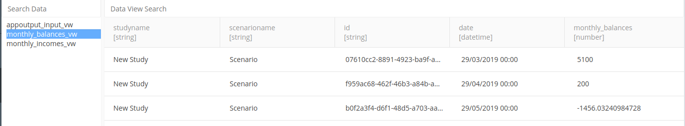
The screen is broken up in to two main sections. The left section lists the “tables” that are generated by the application. Clicking on a table shows the data in the right section. A right click provides functionality to export the whole table (use with caution, as this can cause issues with your browser for large data sets), export the current page, or delete the table. Rerunning the application will recreate it.
The Data View Search box allows the user to search the data set, using a Sql like syntax, eg scenarioname='Scenario' will filter on the scenario called Scenario. Clicking on a column header will sort by that column.
Each column also displays the datatype the data is stored under. This is useful when diagnosing reporting issues and data type errors.
Congratulations! You have now completed your first Akumen model, using either Driver Models, Python or R.
After modelling the coffee shop you should find that the best price for a cup of coffee in John and Jack’s new coffee shop is $3.7 or $3.6 (depending on the distribution results). This is the best value that gives them the best value at the end of 12 months.
This is the end of the coffee shop tutorial. More tutorials have been included in the menu on the left of your screen should you wish to learn more about Driver Models, Python or R.
Welcome to the Linking Python Apps tutorial. This tutorial demonstrates how to link two Python applications together using API calls. Linking applications is useful for creating an ecosystem of micro services, rather than large monolithic applications. This improves the overall efficiency of Akumen, and makes it much easier to test if each application does only one thing and one thing well.
The Akumen API provides a rich set of functions to enable application developers to interact with the Akumen platform. Documentation is available here .
For this tutorial we’ll need two applications. The first (called Master) is a simple application that does very little except provide a single float input value that we’ll access and modify from the second (Slave), as well as generate an output table of random numbers.
The second step is to create the slave application.
All of the code is listed below with full code comments so that once it’s created under your client it can remain as a reference on how Akumen apps can talk to one another.
This application does the following:
Make sure to follow through with “Create Slave App Part 2” or this code will not work!
Once the main.py file is created, we need to access the scenario parameter to point to the master app. This needs to be done from the Slave app.
We use Python requests to be able to make API calls to Akumen. We also need to import akumen_api to access the API url and token. The token is generated by the currently executing user, so best practice is not to hard code your own token in the app, but use the currently executing user’s token. This means that scheduled apps will use the runas user, ensuring security is adhered to.
We need to add the authorization token to the headers of the requests object. This can be done through a dictionary called headers.
And generate a url of the request we want to access, using the details from the incoming input parameter. This could be hardcoded, but by using a scenario parameter, it gives us the flexibility of allowing the users select a scenario. For example, we could have an approved operational scenario they need to run the app against, or a test scenario to validate something.
Now we need to actually run the request. Note that we use a get call here. We could use a post or also delete. Look at the API help for the correct call.
Requests also has additional parameters. If we’re doing a post, and have a json object as part of the request, we need to use json={…} where {…} is a json object to pass in. If it’s a json string, ie json.dumps({…}), we use data=string.
Checking for errors involves checking the response.status_code for 500 or 404. If it’s one of these, we convert the response to json using response_json=json.loads(response.text) and querying the ’error’ object for the actual error. An exception can be raised in this case, which will abort app execution.
Look here for more information on the Python helpers.
This chapter presents a situtation where we need to build a model that utilises machine learning. The model built in this example will help in determining whether a collection of breast tissue samples are maligant or not.
In this example, we work through an example of using Machine Learning in Akumen to classify breast tumour biopsies into two categories: M (malignant) or B (benign). Rather than operating directly on images of the tumours, we instead apply machine learning to a series of quantitative features relating to the images.
The data is publically available here, provided by the University of Wisconsin Clinical Sciences Center.
The Machine Learning model is broken up into a number of key components, derived from freely-available helper apps within Akumen. These components are:
Not every machine learning application needs these four components: some can be three. If you’re training a model to determine accuracy and not execute on an ongoing basis, you can use two.
The data connector is an automated application that retrieves a file, determines its delimited format, and converts into an output datatable. It takes the following parameters:
data_url: a URL to the datafile (csv, tsv, psv or other)delimiter: this can be supplied if required, but will be automatically determined if left blankskiprows: the number of rows to skip before the header line in the datafileskipcols: the number of columns to skip before the first data columnTo create a data connector model, you can do the following:
Create Application -> Python Model, named Connector - Breast Cancer.Git Clone button on the toolbar, and enter the git url: https://gitlab.com/optika-solutions/apps/xsv-http-connector.git. You can leave the username and password blank, but hit the refresh button next to the branch selector, then select the branch master. Click ok.https://s3-ap-southeast-2.amazonaws.com/akumen-public-bucket/data.csv into data_url. All other fields can be left blank.
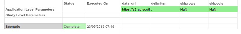
data_vw view in the Data tab to see the loaded data.
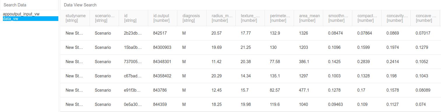
Performing ETL activities consume a significant part of the average data science workflow. With Akumen, we aim to streamline it somewhat by using PETL - a Python ETL library and makes transforms relatively simple. This model is simple, because there isn’t much ETL required for this dataset - it’s all basically in the format that we need. Hence, we just perform some minor transformations to show the workflow.
To create an ETL model, you can do the following:
Create Application -> Python Model, named ETL - Breast Cancer.Dockerfile (which will be created from a template) and add the petl install line as below:main.py and add the following, step-by-step:The first line imports petl, the Python ETL library. The second line imports a helper from Akumen’s API functions, get_results, which retrieves data from another model’s execution. We’ll use this to get the data from our data connector in the previous section.
This section is our standard Akumen wrapper function and parameter definitions. In this model, we take three parameters:
data - a scenario input that points to our Connector model. We use this with get_results to retrieve the connector’s result data (which is our breast cancer data).view - the name of the view that we want to retrieve results from. For our connector, this is data_vw.scope - the scope level that we want to retrieve data for. We’re only retrieving data from a single scenario, so scenario scope is fine.Using get_results, we retrieve the dataset from the Connector model and pass it into petl. get_results returns a dataframe, which is easily imported into petl for modification.
As a simple modification, we reform the diagnosis column into a binary integer format. petl provides a large number of transformation functions that can be used, but other libraries or code can be used here too - fuzzy matching, integration, or others.
We also want to cut off some Akumen-standard columns, so they’re not duplicated by this model.
And we return the resulting dataframe for output.
The entire resulting file is below:
For inputs, you should use:
data: the connector model we previously built.view: data_vwscope: scenario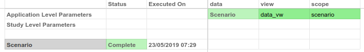
Execute the model and go to the data tab, and you should see that the diagnosis column is now 0/1 instead of B/M.
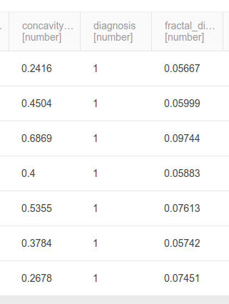
In this section, we use auto-sklearn to train an ensemble ML model to accurately classify tumour rows as malignant or benign. Akumen provides a model to perform this task, that requires some minor configuration. It requires the following parameters:
source: a scenario input, pointing to the dataset to be trained from. For our purposes, this is the ETL model we just wrote.view_name: name of the view to retrieve data from.scope: scope level of the data to retrieve from (see previous section).features: a JSON configuration section that defines the features to train the model with.target: the column that you’re attempting to classify data to.model_type: regression or classification, defines the type of ML to perform.training_split: what percentage of input data to use for training vs testing of the model. The default is 70%, and this is generally fine.We provide support for using either the Akumen Document Manager or a third party cloud storage service for saving the exported data. Examples are provided below for performing either method.
To create an ML training model, you can do the following:
Create Application -> Python Model, named ML Trainer - Breast Cancer.Git Clone button on the toolbar, and enter the git url: https://gitlab.com/optika-solutions/apps/auto-sklearn-trainer-document.git. You can leave the username and password blank, just hit the refresh button next to branch, ensure the branch is on master. Click ok.source: point to the ETL model.scope: scenarioview_name: results_vwfeatures: see below.target: diagnosismodel_type: classificationtraining_split: 0.7For features JSON, we list each column under its associated type. A numeric type is any feature that is numeric-based (number and order is important). A categorical type is any feature in which order is not important, but each distinct value is (e.g. true/false, or colours, or similar). String values must be categorical. To ignore a feature, simply exclude it from this list - however, the model will automatically exclude any features it determines to be irrelevant anyway.
Then we execute the scenario. Once completed, you’ll notice that the model returns an indicative accuracy - in this case, roughly ~95-97%.

If you check the document manager, you’ll also see your model.

Alternatively, you may use AWS or Azure to store the model. The steps below are written using an S3 bucket.
Note: You will need to provide your own Amazon S3 bucket to store the model in AWS.
To create an ML training model using an Amazon S3 bucket, you can do the following:
Create Application -> Python Model, named ML Trainer - Breast Cancer.Git Clone button on the toolbar, and enter the git url: https://gitlab.com/optika-solutions/apps/auto-sklearn-trainer.git. You can leave the username and password blank, just hit the refresh button next to branch, ensure the branch is on master. Click ok.source: point to the ETL model.scope: scenarioview_name: results_vwfeatures: see below.target: diagnosismodel_type: classificationtraining_split: 0.7output_configuration: see below.For features, use the JSON provided above for the previous example.
For the output_configuration JSON below, we give a storage provider and keys (in this case, for S3 - but Azure Blob Storage is also supported).
Note: The name entered into bucket must match an existing s3 bucket in AWS. The key and secret values must also be updated to a valid AWS access key with appropriate permissions to the bucket.
Then we execute the scenario. Once completed, you’ll notice that the model returns an indicative accuracy - in this case, roughly ~95-97%.
If you check the S3 bucket, you’ll also see your model.
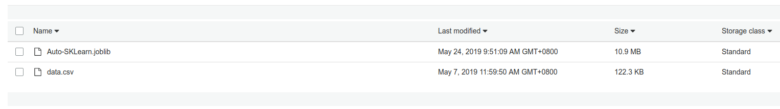
Now that the model is trained, we don’t want to re-train it every time we want to classify or regress data. Because we saved the trained model to the document library, we can retrieve it and execute it against a dataset using an executor model.
The model takes the following parameters:
training_model_name: the name of the model created in the training section of the tutorialtarget: the target column to fill the prediction, or leave blank for default of result.data: tabular data that contains every column used as a feature in the trained model, with as many rows as should be processed.Examples are provided below for retrieving the trained model data from either the Akumen Document Manager or a third party cloud storage service.
To create an ML execution model, you can do the following:
Create Application -> Python Model, named ML Executor - Breast Cancer.Git Clone button on the toolbar, and enter the git url: https://gitlab.com/optika-solutions/apps/auto-sklearn-executor-document.git. You can leave the username and password blank, and the branch on master. Click ok.training_model_name: ML Trainer - Breast Cancertarget: leave blank.data: see below.As a sample, you can use the following for data (Save the contents as a CSV and upload to the data spreadsheet):
Execute the scenario. Once completed, go to the data tab and find the result column.
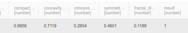
Alternatively, if an Amazon S3 bucket was used for the ML Training model, the steps below can be used to retrieve the data:
The model takes the following parameters:
training_model_name: the name of the model created in the training section of the tutorialjoblib_location: see below.target: the target column to fill the prediction, or leave blank for default of result.data: tabular data that contains every column used as a feature in the trained model, with as many rows as should be processed.joblib_location JSON:
To create an ML execution model, you can do the following:
Create Application -> Python Model, named ML Executor - Breast Cancer.Git Clone button on the toolbar, and enter the git url: https://gitlab.com/optika-solutions/apps/auto-sklearn-executor.git. You can leave the username and password blank, and the branch on master. Click ok.training_model_name: ML Trainer - Breast Cancerjoblib_location: see above.target: leave blank.data: see below.As a sample, you can use the following for data (Save the contents as a CSV and upload to the data spreadsheet):
Execute the scenario. Once completed, go to the data tab and find the result column.
Welcome to the Akumen Pages tutorial. This tutorial will step you through creating a page in Akumen that can be used to manage scenarios and enter data for a given model, and customize that page for your own organization.
Pages in Akumen are anything you want them to be, from a simple iframe to render an external system (or even an Akumen page) within Akumen, to a completely bespoke entry screen for your application.
Three options are available:
In this tutorial, we are going to create a page by template, and linking it to an application. Be sure to have followed the Python or R coffee shop tutorial. Although this works for Driver Models, some further customization may be required in the page due to the sheer number of parameters that can be displayed
The Published checkbox means the page is visible to all users (if they have permissions). Not checking the Published checkbox means general users will not be able to see they page unless they are admins and have permissions to see the page (which they will do by default)
The page editor looks and behaves in exactly the same way as the Python and R editors. It provides the same user experience, only it allows you to add html and javascript to customize the page to your needs. Review the readme file for additional customization options and javascript calls.
We will now modify the html to add a bit more information into the data dictionary
Clicking on the Cog next to the name of the page, then clicking on Configuration provides JSON based configuration options the page can utilise. Review the readme.txt file for information on how to use this configuration.
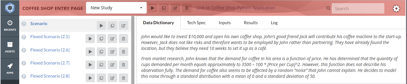
You will notice a number of different components in this page:
The data dictionary should display in italics the content we pasted into the dictionary.html file
This collection of tutorials is focused on taking the information from the Driver Models Section and turning it into examples that users can follow to understand how to put strings of nodes together to build simple Driver Models.
Each tutorial will start off simple, but there will also be a more complex part to each of the examples which will demonstrate how to make Driver Models solver bigger and more complex problems.
Below is a list of the Driver Model tutorials.
Calculation Models are the simplest form of Driver Model. This tutorial demonstrates how to use Numeric nodes and Calculation nodes. It also demonstrates the power of scenario analysis and how to use the Research Grid.
In this tutorial users will be able to build a very simple form of Calculation model, and use the research grid to investigate the results.
This is a very simple Driver Model demonstrating how to put simple Driver Models together using only Calculation and Numeric nodes. This example is not intended for those who know and understand how to put Driver Models together.
To start this tutorial create a new Driver Model in the Apps page. Once the new Driver Model app has been created you will be taken to the build workspace of the Driver Model.
We will start building the driver model by setting up two Numeric nodes:
Two numeric nodes will already be on the workspace with two Calculation nodes when you create a new Driver Model. We will ignore the Calculation nodes for the mean time and focus on the Numeric nodes.
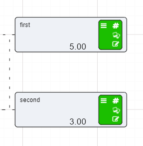
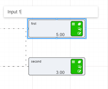
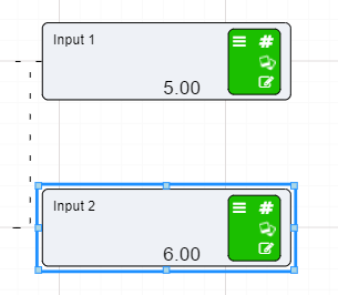
We have no properties to enter for these nodes therefore we can add our Calculation node.
Make sure that the Publish to Results tick box has a tick in it, otherwise when we go to the results tab and try to analyse the results we will not be able to view any of the results generated. The same is true for all nodes in the Driver Model.
Warning
The Calculation node for this example will take the two input values and multiply them together.
Now when the new Driver Model was created, there are already two Calculation nodes attached to two Numeric nodes. We only need one of the Calculation nodes so click on one of the nodes and either:
For the other Calculation node:
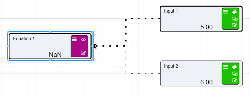
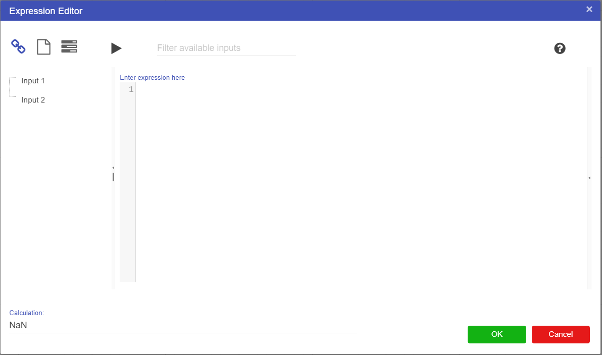
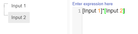
[Input 1]*[Input 2]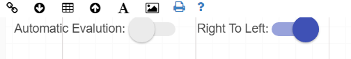
The node will then do the calculation and display the results.
That until an expression is entered into the Expression Editor that involves the attached nodes, the connecting lines will remained dotted. When the node is used in a calculation the lines will become solid when the node calculates the result.
Make sure that the Publish to Results tick box has a tick in it, otherwise when we go to the results tab and try to analyse the results we will not be able to view any of the results generated. The same is true for all nodes in the Driver Model.
The Calculation node is now dependant on the values of the first two Numeric nodes. So if the value of Input 1 changes from 5 to 7, the result of the Calculation node will change too. The results from this model though are not interesting. We have created a model to simulate times tables.
However if we add more nodes to the model, and more Calculation nodes then the results might be more interesting.
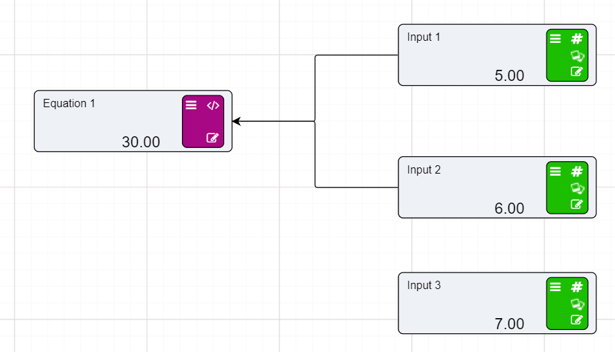
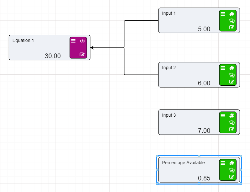
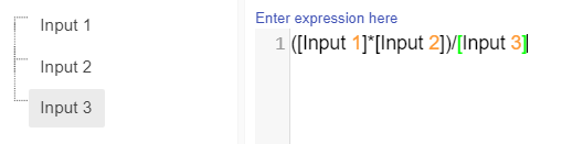
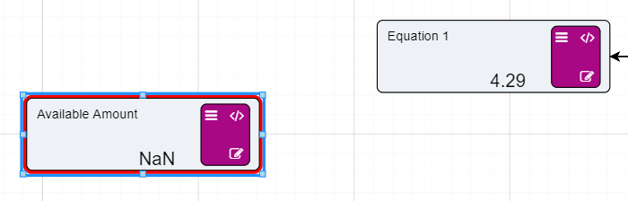
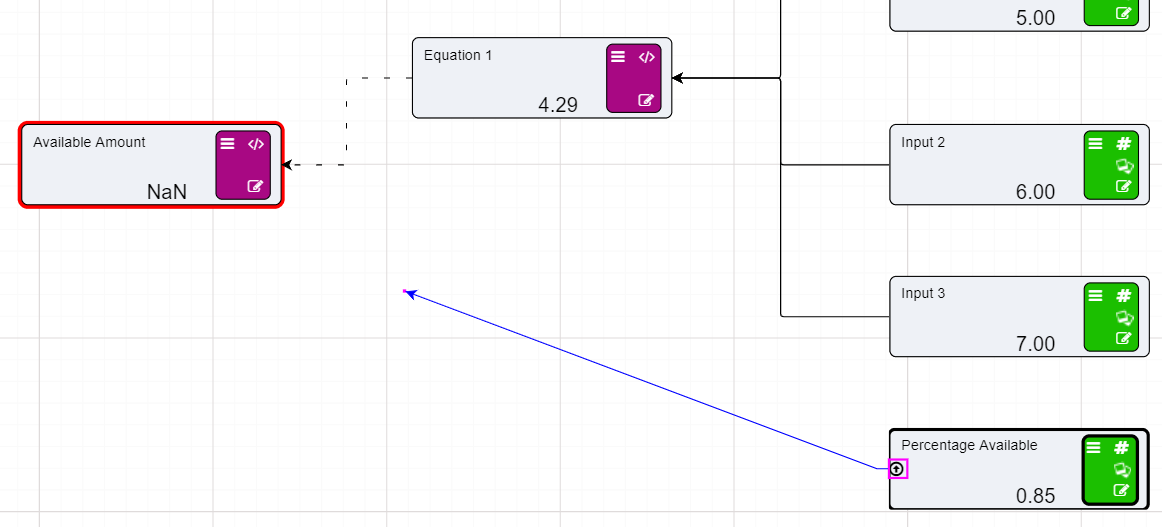
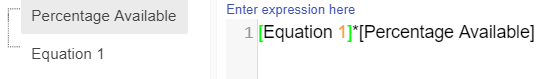
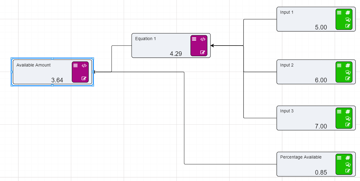 This string of equations allows us to go to the research grid to evaluate and flex the results.
The Research Grid will provide us with the tools to look at the different results produced by the Driver Model. To do this we must generate scenarios by which we can evaluate the results. There are few types of results we could look at. If we assume that we are looking for a value as close to a round number as possible we could change any one of the four values displayed in the Research Grid.
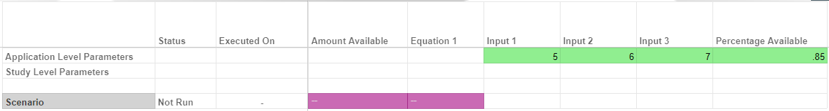
The best way to create these kinds of scenarios is by using the flex function. Flexing will allow us to create a number of scenarios based on the changing values of one or more user inputs.
To generate new scenarios in the Research grid:
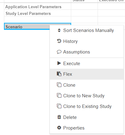
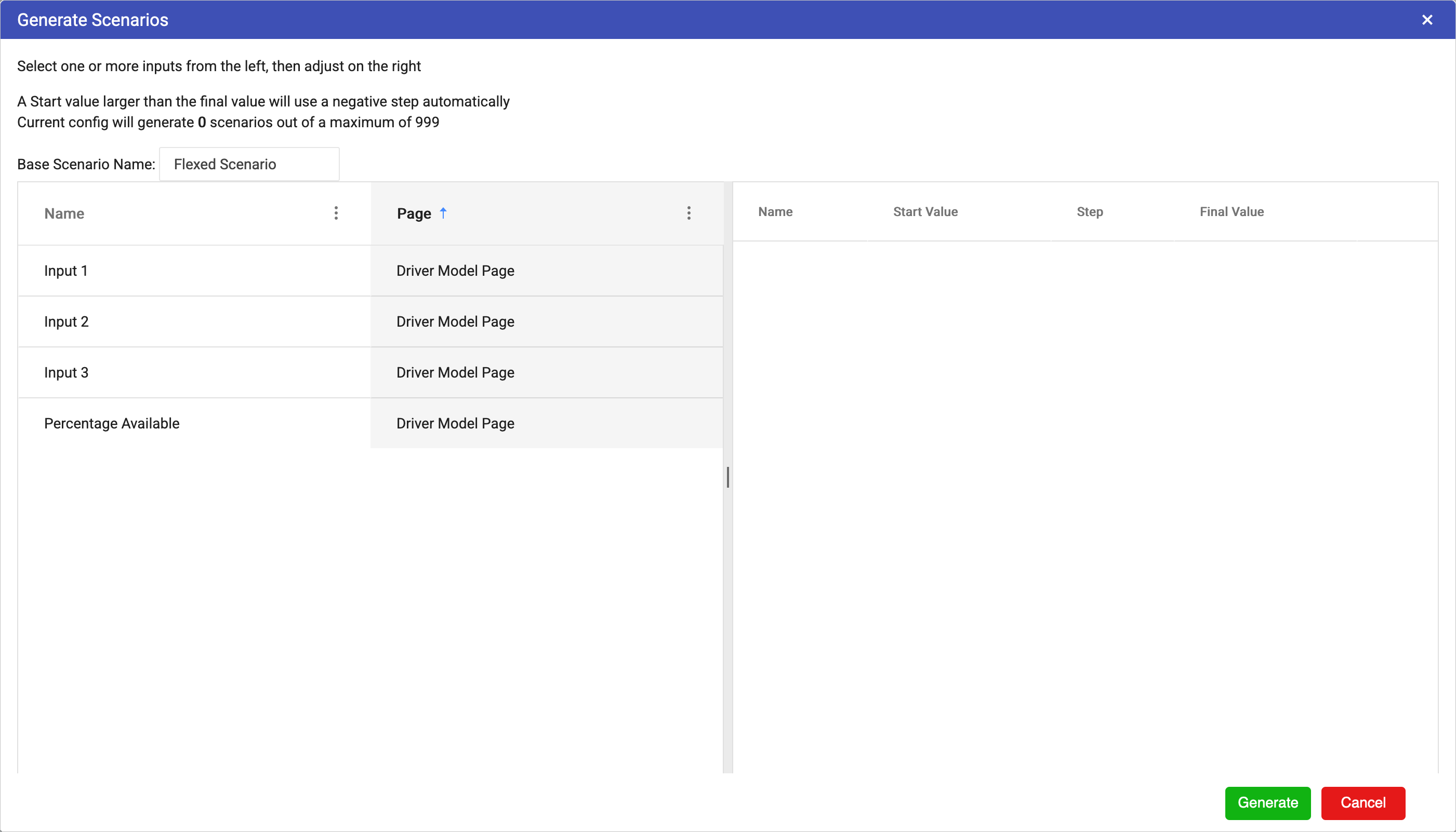
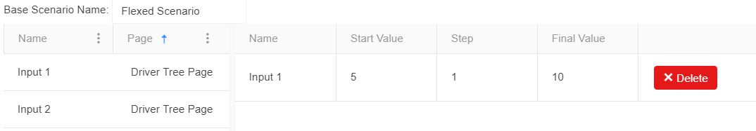 We can flex more than one value at a time so we will also flex Input 2
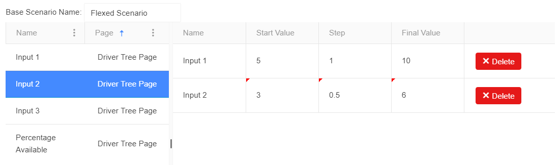
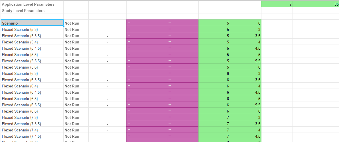
Once all the different scenarios have been generated we can execute them to see the results.
To execute the scenarios:

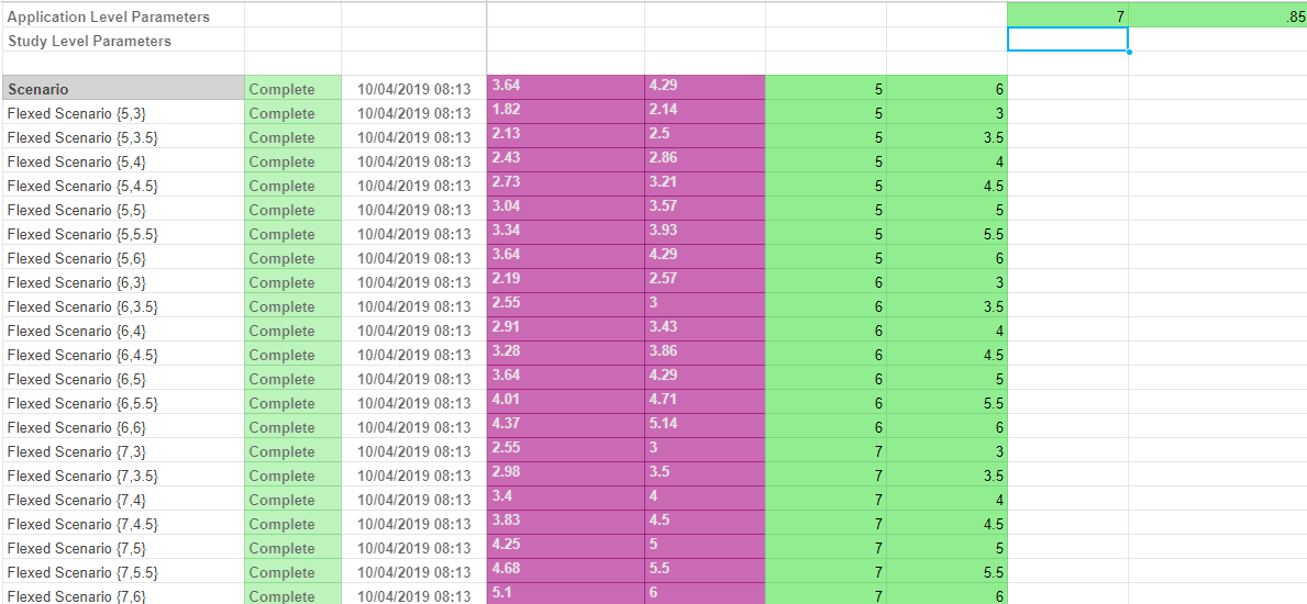
Now that we have executed the scenarios we can see the direct results on the research grid. For a slightly more complex model we would suggest reviewing the results with the help of the Research tab.
In this tutorial we will talk about Asset Parameter nodes and how they fit in a Driver Model and why they are invaluable to Driver Models.
In this tutorial we will be using the example of a mine, though the concepts of this tutorial can be transferred to any model where there are constant concepts central to the running of a business. For more information on the Asset Library click here.
The context for this tutorial is as follows:
There are two truck shifts at a mine site. This mine site wants to track the number of tonnes of material moved in the mine site everyday by these trucks. Three additional trucks have been purchased to increase the availability of the trucks in both shifts but they want to know where the trucks should go to increase the amount of tonnes moved each day.
The main concept in this business is the mine trucks. These mine trucks and their properties cannot be changed and therefore would benefit from having their properties added to the Asset Library.
The following properties will be used in the model and so will be added to the Asset Library:
We will now add the Mine Branch to the Asset Library and the truck Shift Assets.
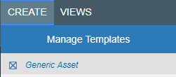
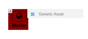
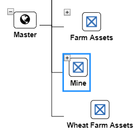
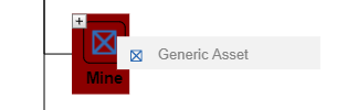
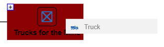
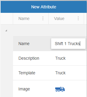
Once all the assets surrounding the Trucks and mine have been added the different properties regarding the truck shifts can be added.
Every asset template comes with a certain set of attributes. Availability is not a preset attribute in the Trucks template so it will need to be added to both of those assets in order for it to be stored in the Asset Library.

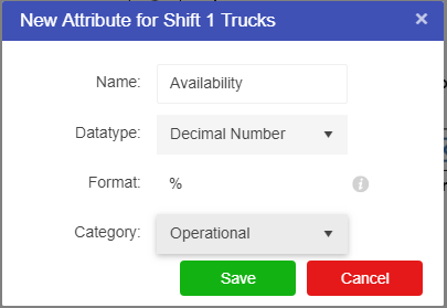
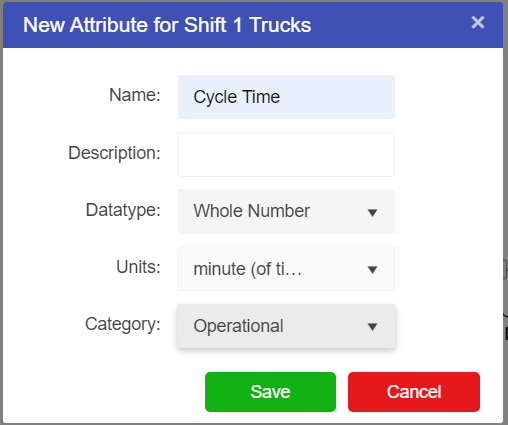
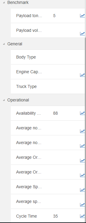
The Truck assets are now ready for use in the Driver Model.
Whenever you change the Datatype of an asset, the format of the values you can enter will change as well. So for example the formats for the Datatype Date/Time will be different to those for the format Decimal Number, and Whole Number will require units instead of a format. To see which formats are allowed hover over the little info circle next to the format box.
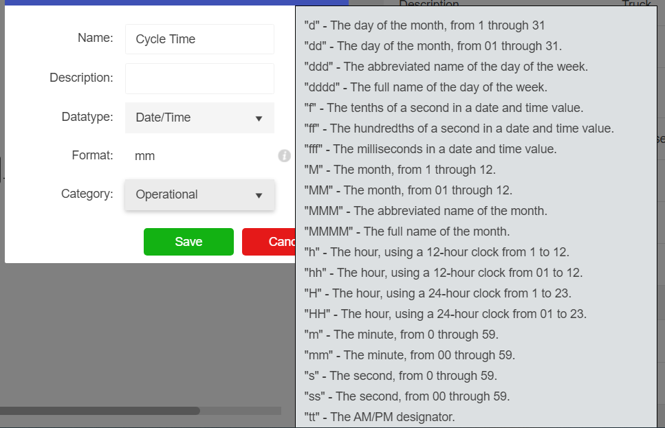
Every time users want to test create a new model they will need to go to the Application Manager (APPS). Click on the APPS button to get to the Application Manager.
To create a new Driver Model, once in APPS:
Users will then be taken to the workspace fo the new driver model.
Pages will help to keep the two truck shifts separate until the end of the Driver Model. We will create two sub pages in this model.
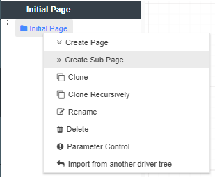
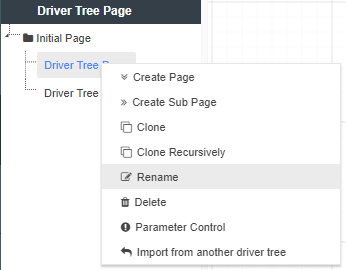
Now we can start creating the Driver Model for Shift 1.
For each of the Shift Driver Models there will be two numeric nodes:
Both of these nodes could have been placed in the Asset Library, but since they are going to change values several times in this tutorial they are better as Numeric nodes since they are easier to change than Asset Parameter nodes.
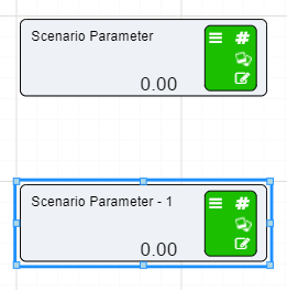
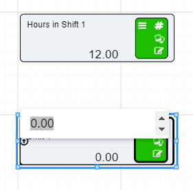
For the Shift 2 sub page the steps are exactly the same, only:
The number of hours in Shift 2 is the same as Shift 1
Asset Parameters nodes are easy to set up as described on the Asset Parameter node page. For this example we will be setting up three Asset Parameter nodes on each of the sub pages. One for:
To set up these nodes:
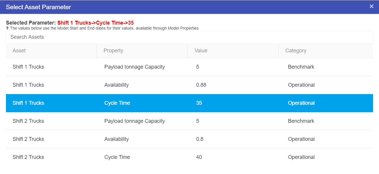
Make sure that for the Asset Parameter nodes on the Shift 2 sub page that the assets you are attaching to those nodes come from the Asset Shift 2 Trucks.
The two shifts are separated by pages. These two pages can be brought together through the use of Node Reference nodes. Once the final values for ore moved during each shift have been calculated we will use the Node Reference node to take the calculated values and work out the total tonnes of ore moved each day.
First we will find the total value of ore tonnes moved each shift. Starting with Shift 1:
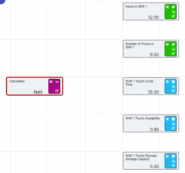
(([Hours in Shift 1]*60)/[Shift 1 Trucks.Cycle Time])*[Shift 1 Trucks.Payload tonnage Capacity]*[Number of Trucks in Shift 1]*[Shift 1 Trucks.Availability]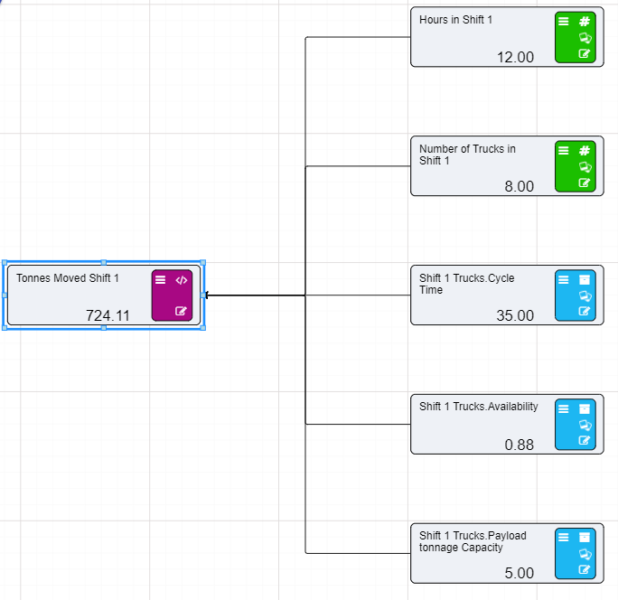
You will need to change Shift 1 in the above expression to Shift 2 if you use copy and paste.
Now that tonnes moved for Shift 1 and Shift 2 have been calculated, the final total can be calculated on the Total Tonnes Moved page using Node Reference nodes.
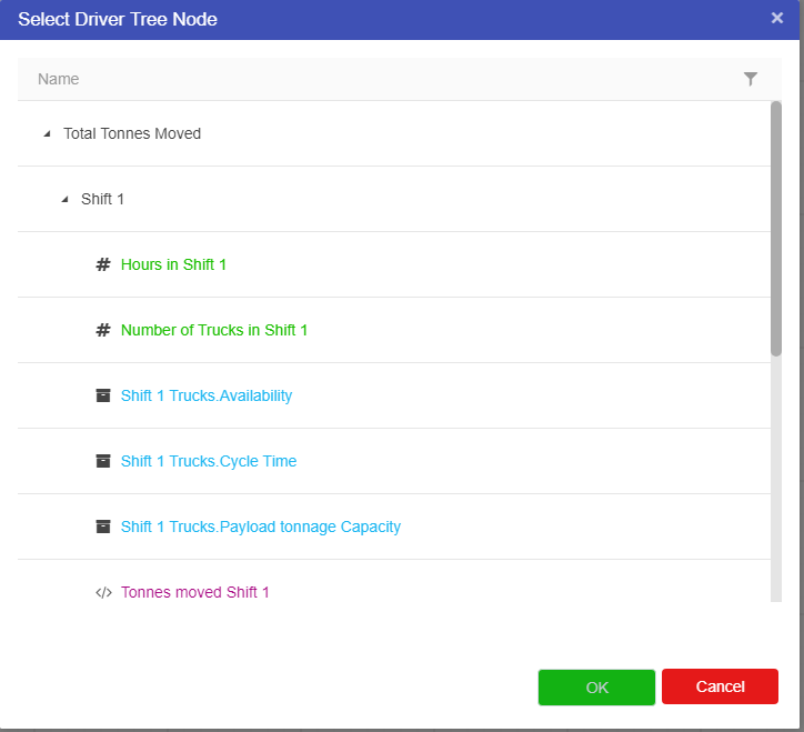
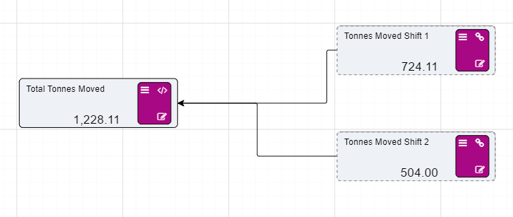
Now that we have calculated the total tonnes of material we can do some research into these two shifts to find out where these two trucks should go to increase or move roughly the same amount of material each day.
We know that the mine has purchased three extra trucks to increase the availability. But they do not know where these trucks should go in order to maximize the amount of ore moved between the two shifts. So where would those three trucks go? What would the results be? This is the kind of research the Akumen can do using its ability to spilt research into Studies.
Adding a truck to each shift changes the availability of the trucks for the shift, since the current availability of how many trucks are avilable on shift is determined by the asset library adding new trucks could change the availability. For Shift 1 it is assumed that each truck is unavilable on average 2% of the time while for Shift 2 each truck is unavailable for 3% of the time.
So first before we can begin our research we need to go into the driver model and set up a calcualtion node to work out the new availability of the trucks.
(100-([Number of Trucks in Shift 1]*2))/100.(([Hours in Shift 1]*60)/[Shift 1 Trucks.Cycle Time])*[Shift 1 Trucks.Payload tonnage Capacity]*[Number of Trucks in Shift 1]*[Availability for Shift 1]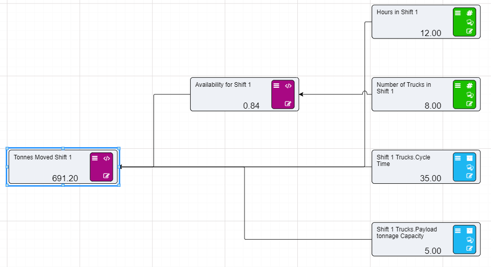
(100-([Number of Trucks in Shift 1]*3))/100.
This is because the percentage of unavilability is different from Shift 1 to that of Shift 2.Now that the Driver Model for the Mine has been modified we can start looking into how the amount of ore moved can be maximized. To do this we need to go to the Research Grid.
The Research Grid will show all of the different nodes in the Driver Model, but the only ones that we can change are the ones that are coloured green. Currently these values are sitting at the top of the Research Grid in the Application Level. We are going to change these values so to see the effects There are two ways we can create new scenarios:
We are going to be using cloning to find the maximum.
We know that there are 3 extra trucks. There can only be three extra trucks in total so we will need to clone a few scenarios. We could use flexing but since we can only have three extra trucks cloning would be easier.
We will need the following scenarios where:
To clone the baseline scenario so we can observe these changes to the number of trucks:
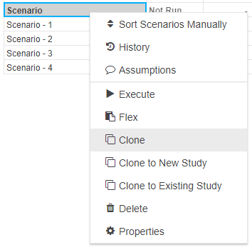
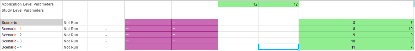
Once the scenarios have been cloned set each scenario up to reflect the list above. Then execute the scenarios.
Once the scenarios have been run we can view the results in the Research, Data, or Reports tab. The immediate results will be visible in the Research tab under the column that says Total Tonnes Moved. You will need to go use the scroll bar to go to the very end of the Research Grid.
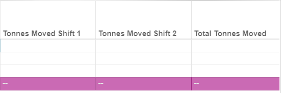
In this tutorial we will discuss how to use three of the more complex nodes, the Prior Value node, the Timeseries node and the Distribution node.
This tutorial will look at how to fit the three nodes together to create a Driver Model that can predict future values. The Driver Model will predict the amount left to pay off on a mortgage for a house.
This model is based off the following scenario:
A finance broker is investigating a home loan for a client. The amount they will have to borrow from the bank with be $160000. The broker has calculated that the repayments each month will be $736, at a variable interest rate of 3.76% per annum which will likely change at a normal rate of 3 std. Before the broker presents this option to the client they want to predict what the loan figure will look like after 12 repayments, just over a year since taking out the loan.
For users wishing to complete this tutorial you will need to create a new Application from the APPS screen and delete the nodes already on the workspace.
The first step for any Driver Model is to set up the required Numeric nodes. They will provide the constant values, values that we will be able to change when we go to the Research Grid.
The two constant values that we have for this driver model are the:
To set up these nodes:
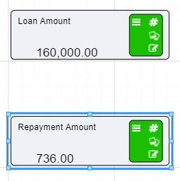
The next node to set up is the Distribution node. The distribution node will be used for the interest rate of the loan. Distribution nodes require several pieces of information:
As mentioned in the tutorial description the interest rate was mentioned to be 3.76% per annum which will likely change at a normal rate of 3 std. Therefore the:
Not all distribution types will be normal. For this example it is assumed to be a normal distribution to mimic the change in interest rates over the course of a year. See the Distribution node page for more information as to the types of distributions the Distribution node supports.
To set up the Distribution node:
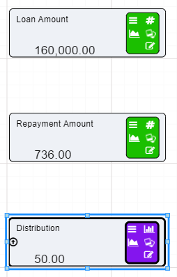
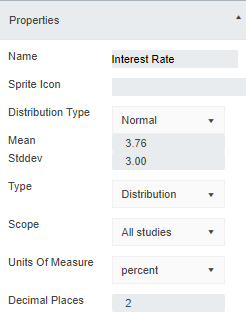
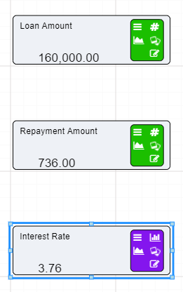
The last thing we need to do is check the number of iterations that the model runs is set to 100. This will ensure that the the model does not hit the hard limit of iterations for the model.
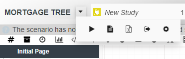
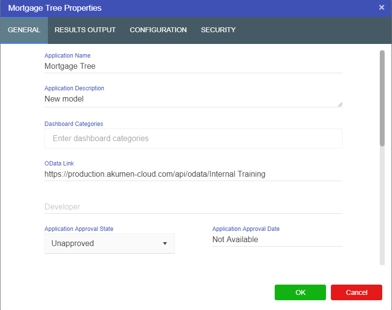
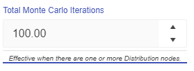
The final node to set up, before the Spreadsheet Input nodes are added, is the Timeseries node. The Timeseries node will allow the model to predict values for the model over a period of time. To set up a Timeseries node users will need to know the:
In this case that period of time is 12 months, therefore, the time step type is months, and there will be 12 of them. Most time steps require the value of each time step as well. For this case we will label the months 1 through to 12.
To set up the Timeseries node:
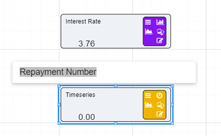
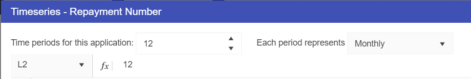
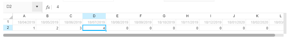
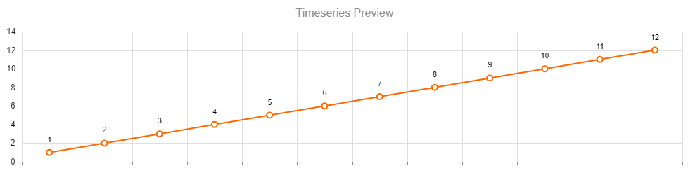
A slider bar will appear at the bottom of the screen. This allows users to go through each time period to see the values that change over time.

The next node we need to set up for this Driver Model is the Prior Value node. The Prior Value node works in conjunction with a Timeseries node. It works by creating a loop which stores a specified node value from a previous timestep to be used in the next one.
Since we want to find out how much of the loan will be left at the end of 12 months we can use the Prior Value node to store the value left on the mortgage at the end of every month. Prior Value nodes have two input slots, The first takes an initial value, and the second takes all values produced by the input node after the initial value. For example we know the initial loan amount is 160000, at the end of the first timestep that value will be different. This final value will be fed into the Prior Value node so that we can use that new value in the next timestep.
To set up the Prior Value node:
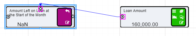
The connecting lines will be dotted until the scenario has run or until the node has been edited, such as setting the node to Publish to Results.
This is all we can currently do to set up the Prior Value node until we have our second input. In the next page we will set up the Calculation nodes we will need to create the true input for the Prior Value node. Once this input is created we can attach the nodes together and view the final result.
For this Driver Model there are going to be 2 Calculation nodes.
First we will set up the equation that will calculate how much interest will be charged per month.
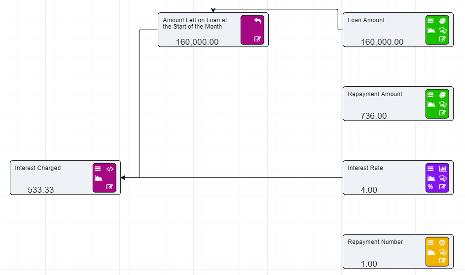
[Amount Left on Loan at the Start of the Month]*([Interest Decimal]/12).
In the above expression we have divided the interest decimal by 12 because the total interest is charged at an annual rate. To get the monthly rate we have to divide the decimal by 12.
For the final Calculation node we have to connect the following three nodes to find the total amount left on the loan at the end of the month.
[Amount Left on Loan at the Start of the Month]+[Interest Charged]-[Repayment Amount].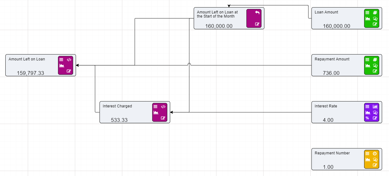
Now that we have set up our Driver Model we can execute our scenario before going to the Research grid to investigate the influence of different inputs.
In this tutorial, we want to examine OEE for our plant. Our plant builds widgets, and we know we have a problem somewhere as we aren’t producing what we expect to produce and keep falling behind in customer orders. In addition, some of our customers are returning widgets saying they are dead on arrival.
A bit of background on our widget plant - we run 3 shifts a day at 7 hours a shift. Each shift has a 30 minute break during the shift, and there is a handover time between shifts of 30 minutes. We only produce widgets, there is no changeover of parts during production. We also know that over a 24 hour period, we are repairing machinery on average 4 hours a day. We know we can produce around 60 widgets a minute, which, based on the 21 hours we expect to operate, is 75600 widgets in a day. But we only produced 51200. Out of those widgets, our customers are returning 8000 of them as dead.
To analyse this, we’ll put together a Value Driver Model.
OEE, or Operational Equipment Effectiveness is a percentage figure comparing what could be produced in the process against what is actually being produced. The OEE calculation is Availability * Performance * Quality.
The driver model will start off with a single OEE node that we will then continually break down into constituent nodes. We will then run what if scenarios to determine the best course of action to improve our OEE, and hopefully meet our customer’s orders to a higher quality.
[Availability] * [Performance] * [Quality]The driver model should look as follows:
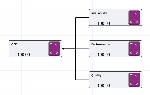
You will notice that all the nodes are calculations - this indicates that we need to break these nodes down further into their constituent parts until we finally get to the raw inputs. These raw inputs become the levers that we can play with to improve our OEE.
To calculate availability, we can use Run Time / Planned Production Time, where Run Time is the Planned Production Time minus any outages.
[Run Time] / [Planned Production Time]. You will notice that the OEE and availability calculations now error out. That is because Run Time and Planned Production Times have no calculations. [Number of Shifts] * ( [Total Shift Length] - [Shift Break])[Planned Production Time] - [Breakdown Time]The driver model should look as follows:
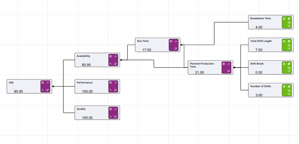
Performance is calculated using (Total Count (including defective items) / Run Time) / Ideal Run Rate. We already have the Run Time, so we reuse that node in the calculation.
([Total Count] / [Run Time]) / [Ideal Run Rate]But hang on - if our runtime is 17 hours, technically we should produce 61,200 widgets, not 51,200. This metric also takes into account slow running, where we are still running, but not as fast as we expect.
The driver model should look like
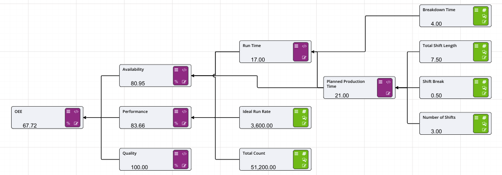
Quality is the number of parts that do not meet quality standards, and is calculated by Good Count / Total Count.
We already have Total Count, and we know that 8000 were returned dead.
[Total Count] - [Dead Widgets][Good Widgets] / [Total Count]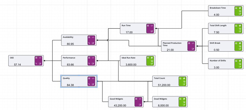
We can see from our driver model that our effectiveness (OEE) is only 57%. Our availability, quality and performance numbers are all above 80%, which on the surface looks ok, but we aren’t really that effective at producing widgets.
That is our baseline scenario. We now want to investigate different scenarios to see which “levers” we can pull to increase our OEE. While it’s possible to simply adjust the numbers in the driver model, it does not provide us a capability of comparing numbers against each other.
But first, so we can create some meaningful reports and compare scenarios, we need to set OEE, Availability, Performance and Quality to publish to results, as shown here. We also want to set the parameter group to results to ensure they are grouped together within the research grid.
Now switch to the Research grid. Notice that because we haven’t “Executed” the scenario, we don’t see any results in the grid. This is different from the Build screen with automatic evaluation turned on. Run the model through the blue Play button at the top.
We now want to see how our metrics change as we adjust different levels.
First we’ll adjust shifts - clone the baseline scenario twice, and call one 2 Shifts and the other 4 Shifts, then alter the shifts in each of those scenarios. You’ll notice the baseline of 3 will move from the application level to the scenario level. We’ll also need to reduce the shift length for 4 shifts, as there’s not enough hours in the day. Change this value to 5.5 for the 4 shift scenario.
Run the model and see what the difference is.
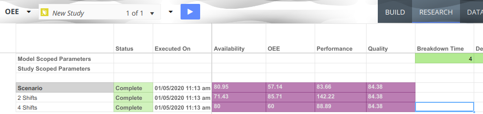
Note that increasing the number of shifts to 4 has led to a minor improvement in OEE, the most improvement we see is from 2 shifts. But drilling down further shows our performance is 142% which is definitely not attainable. Lets increase the shift length, but because of the longer shift length, we need to increase the shift break.
Clone the 2 Shifts scenario, and set the shift length to 11 hours and shift break to 1 hour.
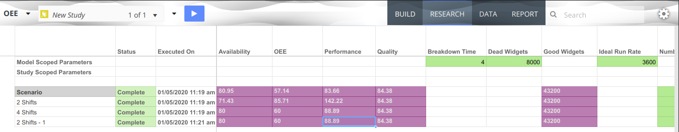
Wow, that gives us the same figure as 4 shifts. Does that mean we could potentially reduce our workforce by 1/3 AND be more effective?
The next thing we might want to look at is improving quality. What if we could reduce the number of dead widgets by half by reducing our run rate to focus more on quality. Lets perform a flex on these two factors.
Right click on the baseline scenario, and hit Flex. Set the Base Scenario Name to Quality Select Dead Widgets, and set step to 500, and final value at 4000. Select Ideal Run Rate and set the step to 250 and Final Value of 2000 Hit Generate then ok. A large number of scenarios should be generated
We also know we want to know the best OEE. We can ask Akumen to order the scenario list after execution by best OEE. Got to the Study Properties and Select the Icon that looks like a Sort icon (tooltip appears saying Allows the user to reorder the scenario by results).
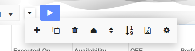
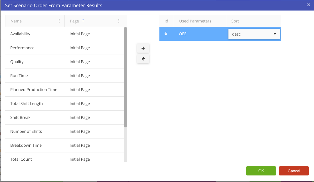
Run the entire set of scenarios by hitting the Play button at the top of the screen. It might take a few minutes to run all those scenarios.
The best OEE will appear at the top once all the scenarios have run.
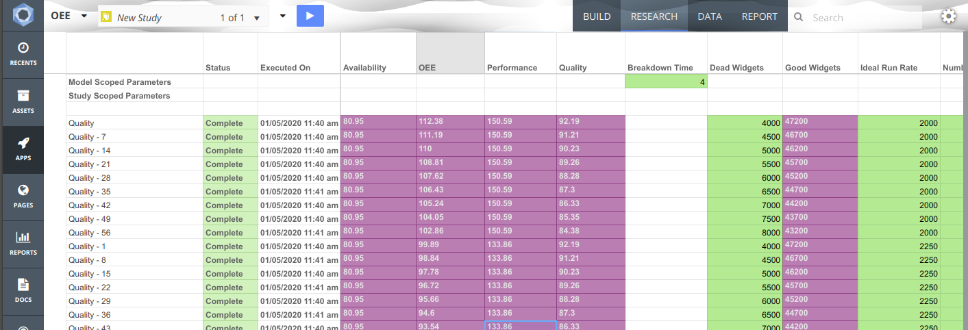
We can now walk through the list, and discard those scenarios (by deleting) te ones that don’t make sense, eg when some of the figures are well above 100%.
Delete all the scenarios at the top of the list by clicking and dragging so they’re highlight. Delete those where the OEE is > 100. In this example it is Quality - 52.
As you can see, we can use a combination of cloning scenarios and adjusting different levers that we can then action.
Finally lets compare these results in a bar chart so we can easily compare them against each other.
Click on the Reports tab and create a Driver Model Report. Click here for more information on how to create a report.
Set the name to OEE Analysis, the Chart Type should be Bar, Parameter Group should be results and we want scenarioname in the X Axis. Finally we want OEE, Availability, Performance and Quality in the Y Axis.
Click ok and we should have a new bar chart appear. By default, it only shows 1 scenario, we can add more scenarios by clicking into the Study/Scenario box.
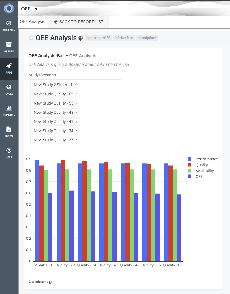
In this example, we have a supply chain with a mine, crusher, rail and port. We’re getting times where the crusher needs to be shutdown and we don’t know why - there is plenty of ore coming from the mine.
Firstly, create a new Driver Model called Debottlenecking.
The first thing we need to do is change the driver model from Right To Left by hitting the toggle At the top of the build screen - we want the nodes to go from left to right to simulate a supply chain.
Now go to the properties of the Model (drop down next to the model name) and set the number of periods to 14 and the reporting period to Daily. We’re basically looking ahead 2 weeks.
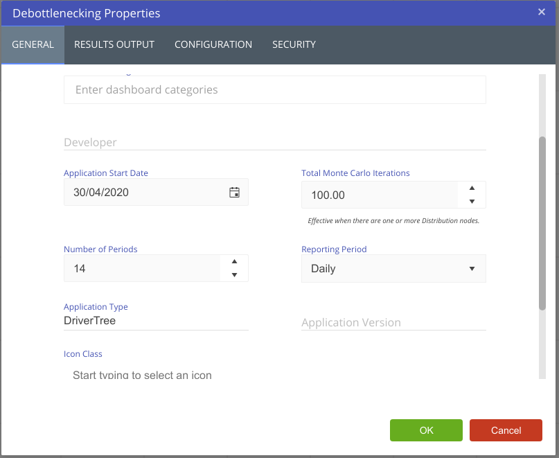
Lets build the mine.
Note that we haven’t yet populated the calculations yet - we need additional node values from the crusher, which we’ll build next.
Lastly we need to connect the output of the Mine Closing balance back into the input of the Mine.
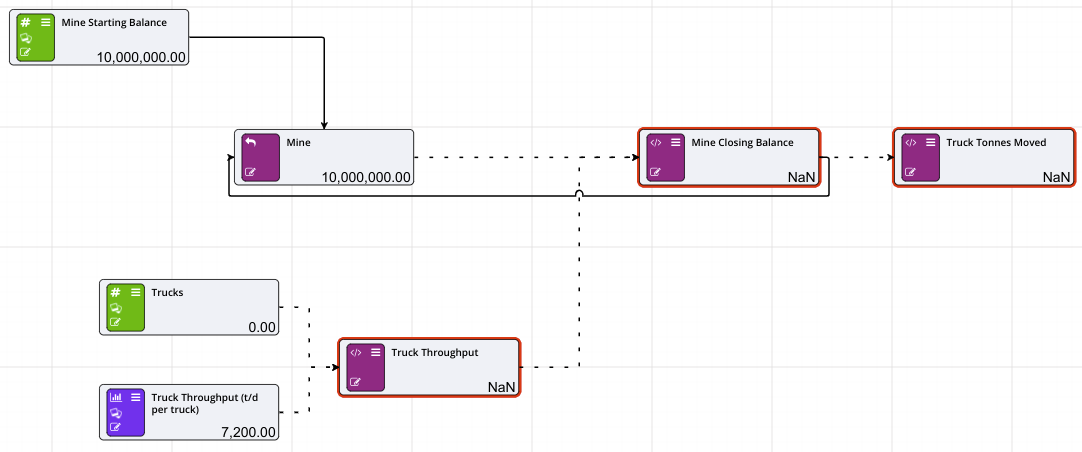
Rename Initial Page in the pages list to Mine by right clicking and hitting Rename. We’ll create each area of our supply chain in a new page.
The layout of the crusher and the rail both follow a very similar pattern to the mine. Lets right click the Mine page and create a new page, renaming it to Crusher.
Now that the first part of the crusher is built, we can go back to the Mine and fill in the calculations.
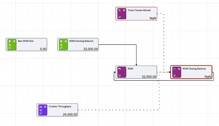
[Mine] - [Truck Throughput]if ([Mine] - [Mine Closing Balance] < 0, 0, [Mine] - [Mine Closing Balance])if ([ROM] + ([Truck Throughput (t/d per truck)] * [Trucks]) >= [Max ROM Size], 0, [Truck Throughput (t/d per truck)]*[Trucks])The Mine page (with Automatic Evaluation on) should look like:
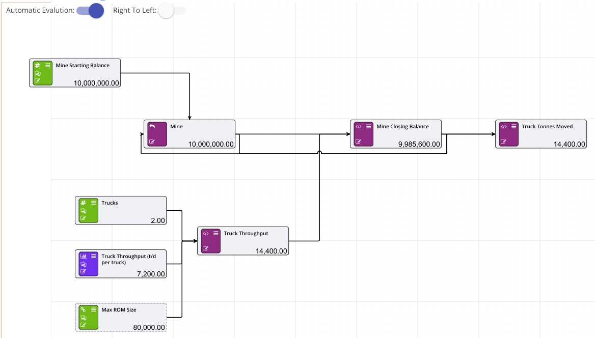
We now need to build the second part of the crusher, a stockpile for the crushed ore.
Create a new numeric node for Stockpile Maximum Size and a value of 200,000
Create a new numeric node for Stockpile Starting Balance and a value of 34,000
Create a new calculation node called Actual Crusher Throughput - this is where we figure out if we can crush ore due to the constraints of the maximum stockpile size. Point Crusher Throughput distribution and Stockpile Maximum size to this node, then Actual Crusher throughput points to ROM Closing Balance. The calculation for this should be if ([Stockpile] + ([Crusher Throughput]) >= [Stockpile Maximum Size], 0, if ([ROM] <= 0, 0, [Crusher Throughput]))
Now update the ROM Closing Balance calculation using the calculation if ([ROM] + [Truck Tonnes Moved] - [Actual Crusher Throughput] < 0, 0, [ROM] + [Truck Tonnes Moved] - [Actual Crusher Throughput])
Create a Prior Value node called Stockpile, with the Stockpile Starting balance feeding into the top initialisation port of the Prior Value node.
Create a Calculation node to the right of the Stockpile node called Stockpile Closing Balance, link the Stockpile node to it, and link the Closing Balance node back into the input of the Stockpile node.
Connect Actual Crusher Throughput to Stockpile Closing Balance.
The crusher should now look like:
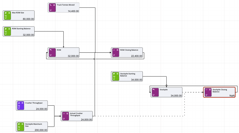
Note that we haven’t yet filled in the Stockpile Closing Balance calculation - we rely on a node from the port, which we haven’t yet set up.
The final steps in the model is to build the rail. Note that this does not model a rail network - we’re only interested in the fact that a train will arrive at certain days of the week to take ore from the stockpile, and drop that ore into another stockpile.
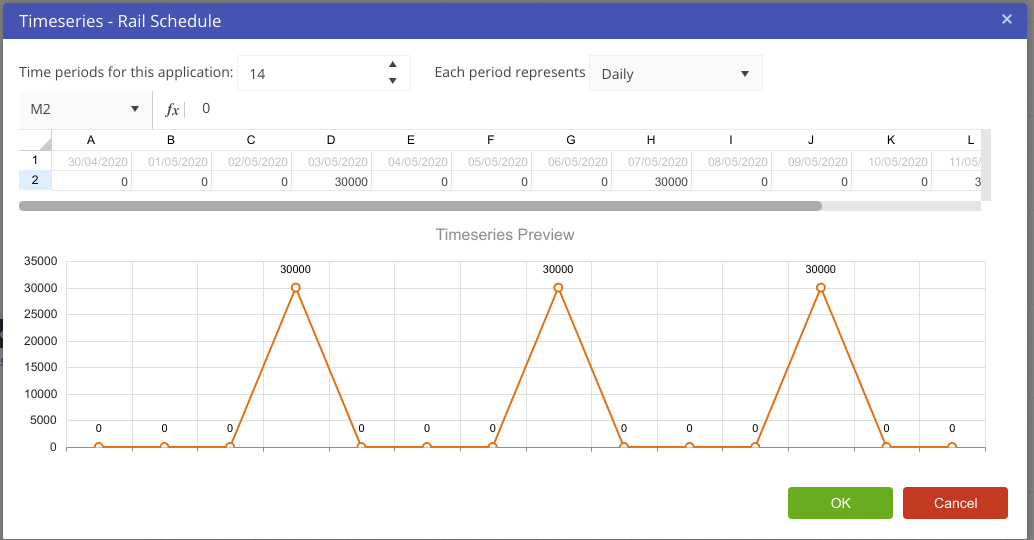
[Stockpile] + [Actual Crusher Throughput] - [Railed Tonnes] for the calculation. The final Crusher page should look as follows: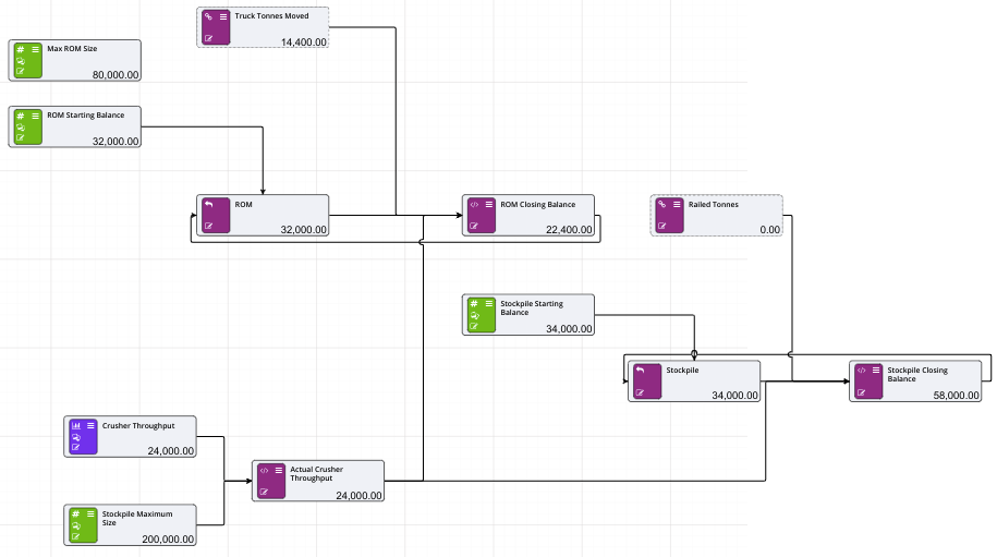
The rail page should look as follows:
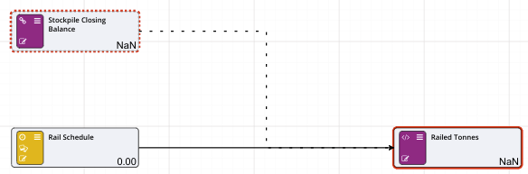
The last stage in the build process for this tutorial is to build the port.
if ([Port Stockpile Opening Balance] + [Rail Schedule] >= [Max Port Stockpile Size], 0, if ([Stockpile Opening Balance] - [Rail Schedule] < 0, 0, [Rail Schedule] ) )The Rail page should now look like:
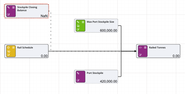
if ([Port Stockpile Opening Balance] - [Ship Schedule] < 0, 0, [Ship Schedule] )[Shipped]+[Shipped Tonnes][Port Stockpile]+[Railed Tonnes]-[Shipped Tonnes]The Port page should look like:
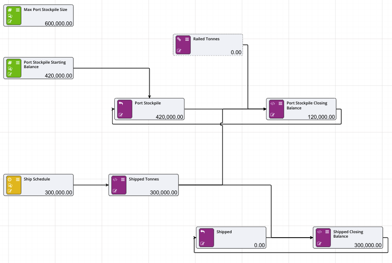
That concludes the build part of the driver model. The next step involves stepping through time and finding where we have issues with our supply chain.
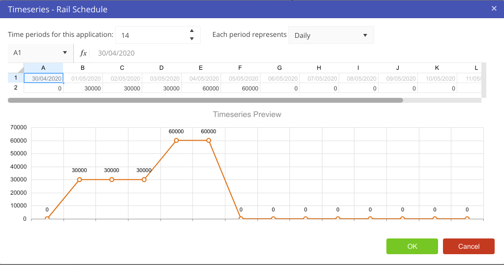
As you can see, every action you take has an effect somewhere within the supply chain. It takes an intense understanding of your own process, but with the power of Akumen at your disposal, you can examine different scenarios to get the most of out of your process, without investing heavily in infrastructure that may or may not work, or have unintended consequences.